Hydrological Analysis
- AverageFlowpathSlope
- AverageUpslopeFlowpathLength
- Basins
- BreachDepressions
- BreachDepressionsLeastCost
- BreachSingleCellPits
- BurnStreamsAtRoads
- D8FlowAccumulation
- D8MassFlux
- D8Pointer
- DInfFlowAccumulation
- DInfMassFlux
- DInfPointer
- DepthInSink
- DepthToWater
- DownslopeDistanceToStream
- DownslopeFlowpathLength
- EdgeContamination
- ElevationAboveStream
- ElevationAboveStreamEuclidean
- Fd8FlowAccumulation
- Fd8Pointer
- FillBurn
- FillDepressions
- FillDepressionsPlanchonAndDarboux
- FillDepressionsWangAndLiu
- FillSingleCellPits
- FindNoFlowCells
- FindParallelFlow
- FlattenLakes
- FloodOrder
- FlowAccumulationFullWorkflow
- FlowLengthDiff
- Hillslopes
- HydrologicConnectivity
- ImpoundmentSizeIndex
- InsertDams
- Isobasins
- JensonSnapPourPoints
- LongestFlowpath
- LowPointsOnHeadwaterDivides
- MaxUpslopeFlowpathLength
- MaxUpslopeValue
- MdInfFlowAccumulation
- NumInflowingNeighbours
- QinFlowAccumulation
- QuinnFlowAccumulation
- RaiseWalls
- Rho8FlowAccumulation
- Rho8Pointer
- RiverCenterlines
- Sink
- SnapPourPoints
- StochasticDepressionAnalysis
- StrahlerOrderBasins
- Subbasins
- TopologicalBreachBurn
- TraceDownslopeFlowpaths
- UnnestBasins
- UpslopeDepressionStorage
- Watershed
AverageFlowpathSlope
This tool calculates the average slope gradient (i.e. slope steepness in degrees) of the flowpaths that
pass through each grid cell in an input digital elevation model (DEM). The user must specify the name of
a DEM raster (--dem). It is important that this DEM is pre-processed to remove all topographic depressions and
flat areas using a tool such as BreachDepressions. Several intermediate rasters are created and stored in
memory during the operation of this tool, which may limit the size of DEM that can be processed, depending
on available system resources.
See Also: AverageUpslopeFlowpathLength, BreachDepressions
Parameters:
| Flag | Description |
|---|---|
| -i, --dem | Input raster DEM file |
| -o, --output | Output raster file |
Python function:
wbt.average_flowpath_slope(
    dem,
    output,
    callback=default_callback
)
Command-line Interface:
>>./whitebox_tools -r=AverageFlowpathSlope -v ^
--wd="/path/to/data/" -i=DEM.tif -o=output.tif
Author: Dr. John Lindsay
Created: 22/07/2017
Last Modified: 17/01/2019
AverageUpslopeFlowpathLength
This tool calculates the average length of the flowpaths that run through each grid cell (in map horizontal units)
in in an input digital elevation model (DEM). The user must specify the name of
a DEM raster (--dem). It is important that this DEM is pre-processed to remove all topographic depressions and
flat areas using a tool such as BreachDepressions. Several intermediate rasters are created and stored in
memory during the operation of this tool, which may limit the size of DEM that can be processed, depending
on available system resources.
See Also: MaxUpslopeFlowpathLength, AverageFlowpathSlope, BreachDepressions
Parameters:
| Flag | Description |
|---|---|
| -i, --dem | Input raster DEM file |
| -o, --output | Output raster file |
Python function:
wbt.average_upslope_flowpath_length(
    dem,
    output,
    callback=default_callback
)
Command-line Interface:
>>./whitebox_tools -r=AverageUpslopeFlowpathLength -v ^
--wd="/path/to/data/" -i=DEM.tif -o=output.tif
Author: Dr. John Lindsay
Created: 25/07/2017
Last Modified: 17/01/2019
Basins
This tool can be used to delineate all of the drainage basins contained within a local drainage direction,
or flow pointer raster (--d8_pntr), and draining to the edge of the data. The flow pointer raster must be derived using
the D8Pointer tool and should have been extracted from a digital elevation model (DEM) that has been
hydrologically pre-processed to remove topographic depressions and flat areas, e.g. using the BreachDepressions
tool. By default, the flow pointer raster is assumed to use the clockwise indexing method used by WhiteboxTools:
| . | . | . |
|---|---|---|
| 64 | 128 | 1 |
| 32 | 0 | 2 |
| 16 | 8 | 4 |
If the pointer file contains ESRI flow direction values instead, the --esri_pntr parameter must be specified.
The Basins and Watershed tools are similar in function but while the Watershed tool identifies the upslope areas that drain to one or more user-specified outlet points, the Basins tool automatically sets outlets to all grid cells situated along the edge of the data that do not have a defined flow direction (i.e. they do not have a lower neighbour). Notice that these edge outlets need not be situated along the edges of the flow-pointer raster, but rather along the edges of the region of valid data. That is, the DEM from which the flow-pointer has been extracted may incompletely fill the containing raster, if it is irregular shaped, and NoData regions may occupy the peripherals. Thus, the entire region of valid data in the flow pointer raster will be divided into a set of mutually exclusive basins using this tool.
See Also: Watershed, D8Pointer, BreachDepressions
Parameters:
| Flag | Description |
|---|---|
| --d8_pntr | Input raster D8 pointer file |
| -o, --output | Output raster file |
| --esri_pntr | D8 pointer uses the ESRI style scheme |
Python function:
wbt.basins(
    d8_pntr,
    output,
    esri_pntr=False,
    callback=default_callback
)
Command-line Interface:
>>./whitebox_tools -r=Basins -v --wd="/path/to/data/" ^
--d8_pntr='d8pntr.tif' -o='output.tif'
Author: Dr. John Lindsay
Created: 01/07/2017
Last Modified: 18/10/2019
BreachDepressions
This tool can be used to remove the depressions in a digital elevation model (DEM), a common requirement of spatial hydrological operations such as flow accumulation and watershed modelling. The tool based on the efficient hybrid depression breaching algorithm described by Lindsay (2016). It uses a breach-first, fill-second approach to resolving continuous flowpaths through depressions.
Notice that when the input DEM (--dem) contains deep, single-cell pits, it can be useful
to raise the pits elevation to that of the lowest neighbour (--fill_pits), to avoid the
creation of deep breach trenches. Deep pits can be common in DEMs containing speckle-type noise.
This option, however, does add slightly to the computation time of the tool.
The user may optionally (--flat_increment) override the default value applied to increment elevations on
flat areas (often formed by the subsequent depression filling operation). The default value is
dependent upon the elevation range in the input DEM and is generally a very small elevation value (e.g.
0.001). It may be necessary to override the default elevation increment value in landscapes where there
are extensive flat areas resulting from depression filling (and along breach channels). Values in the range
0.00001 to 0.01 are generally appropriate. increment values that are too large can result in obvious artifacts
along flattened sites, which may extend beyond the flats, and values that are too small (i.e. smaller than the
numerical precision) may result in the presence of grid cells with no downslope neighbour in the
output DEM. The output DEM will always use 64-bit floating point values for storing elevations because of
the need to precisely represent small elevation differences along flats. Therefore, if the input DEM is stored
at a lower level of precision (e.g. 32-bit floating point elevations), this may result in a doubling of
the size of the DEM.
In comparison with the BreachDepressionsLeastCost tool, this breaching method often provides a less satisfactory, higher impact, breaching solution and is often less efficient. It has been provided to users for legacy reasons and it is advisable that users try the BreachDepressionsLeastCost tool to remove depressions from their DEMs first. The BreachDepressionsLeastCost tool is particularly well suited to breaching through road embankments. Nonetheless, there are applications for which full depression filling using the FillDepressions tool may be preferred.
Reference:
Lindsay JB. 2016. Efficient hybrid breaching-filling sink removal methods for flow path enforcement in digital elevation models. Hydrological Processes, 30(6): 846–857. DOI: 10.1002/hyp.10648
See Also: BreachDepressionsLeastCost, FillDepressions, FillSingleCellPits
Parameters:
| Flag | Description |
|---|---|
| -i, --dem | Input raster DEM file |
| -o, --output | Output raster file |
| --max_depth | Optional maximum breach depth (default is Inf) |
| --max_length | Optional maximum breach channel length (in grid cells; default is Inf) |
| --flat_increment | Optional elevation increment applied to flat areas |
| --fill_pits | Optional flag indicating whether to fill single-cell pits |
Python function:
wbt.breach_depressions(
    dem,
    output,
    max_depth=None,
    max_length=None,
    flat_increment=None,
    fill_pits=False,
    callback=default_callback
)
Command-line Interface:
>>./whitebox_tools -r=BreachDepressions -v ^
--wd="/path/to/data/" --dem=DEM.tif -o=output.tif
Author: Dr. John Lindsay
Created: 28/06/2017
Last Modified: 24/11/2019
BreachDepressionsLeastCost
This tool can be used to perform a type of optimal depression breaching to prepare a digital elevation model (DEM) for hydrological analysis. Depression breaching is a common alternative to depression filling (FillDepressions) and often offers a lower-impact solution to the removal of topographic depressions. This tool implements a method that is loosely based on the algorithm described by Lindsay and Dhun (2015), furthering the earlier algorithm with efficiency optimizations and other significant enhancements. The approach uses a least-cost path analysis to identify the breach channel that connects pit cells (i.e. grid cells for which there is no lower neighbour) to some distant lower cell. Prior to breaching and in order to minimize the depth of breach channels, all pit cells are rised to the elevation of the lowest neighbour minus a small heigh value. Here, the cost of a breach path is determined by the amount of elevation lowering needed to cut the breach channel through the surrounding topography.
The user must specify the name of the input DEM file (--dem), the output breached DEM
file (--output), the maximum search window radius (--dist), the optional maximum breach
cost (--max_cost), and an optional flat height increment value (--flat_increment). Notice that if the
--flat_increment parameter is not specified, the small number used to ensure flow across flats will be
calculated automatically, which should be preferred in most applications of the tool.
The tool operates by performing a least-cost path analysis for each pit cell, radiating outward
until the operation identifies a potential breach destination cell or reaches the maximum breach length parameter.
If a value is specified for the optional --max_cost parameter, then least-cost breach paths that would require
digging a channel that is more costly than this value will be left unbreached. The flat increment value is used
to ensure that there is a monotonically descending path along breach channels to satisfy the necessary
condition of a downslope gradient for flowpath modelling. It is best for this value to be a small
value. If left unspecified, the tool with determine an appropriate value based on the range of
elevation values in the input DEM, which should be the case in most applications. Notice that the need to specify these very small elevation
increment values is one of the reasons why the output DEM will always be of a 64-bit floating-point
data type, which will often double the storage requirements of a DEM (DEMs are often store with 32-bit
precision). Lastly, the user may optionally choose to apply depression filling (--fill) on any depressions
that remain unresolved by the earlier depression breaching operation. This filling step uses an efficient
filling method based on flooding depressions from their pit cells until outlets are identified and then
raising the elevations of flooded cells back and away from the outlets.
The tool can be run in two modes, based on whether the --min_dist is specified. If the --min_dist flag
is specified, the accumulated cost (accum2) of breaching from cell1 to cell2 along a channel
issuing from pit is calculated using the traditional cost-distance function:
cost1 = z1 - (zpit + l × s)
cost2 = z2 - [zpit + (l + 1)s]
accum2 = accum1 + g(cost1 + cost2) / 2.0
where cost1 and cost2 are the costs associated with moving through cell1 and cell2
respectively, z1 and z2 are the elevations of the two cells, zpit is the elevation
of the pit cell, l is the length of the breach channel to cell1, g is the grid cell distance between
cells (accounting for diagonal distances), and s is the small number used to ensure flow
across flats. If the --min_dist flag is not present, the accumulated cost is calculated as:
accum2 = accum1 + cost2
That is, without the --min_dist flag, the tool works to minimize elevation changes to the DEM caused by
breaching, without considering the distance of breach channels. Notice that the value --max_cost, if
specified, should account for this difference in the way cost/cost-distances are calculated. The first cell
in the least-cost accumulation operation that is identified for which cost2 <= 0.0 is the target
cell to which the breach channel will connect the pit along the least-cost path.
In comparison with the BreachDepressions tool, this breaching method often provides a more
satisfactory, lower impact, breaching solution and is often more efficient. It is therefore advisable that users
try the BreachDepressionsLeastCost tool to remove depressions from their DEMs first. This tool is particularly
well suited to breaching through road embankments. There are instances when a breaching solution is inappropriate, e.g.
when a very deep depression such as an open-pit mine occurs in the DEM and long, deep breach paths are created. Often
restricting breaching with the --max_cost parameter, combined with subsequent depression filling (--fill) can
provide an adequate solution in these cases. Nonetheless, there are applications for which full depression filling
using the FillDepressions tool may be preferred.
Reference:
Lindsay J, Dhun K. 2015. Modelling surface drainage patterns in altered landscapes using LiDAR. International Journal of Geographical Information Science, 29: 1-15. DOI: 10.1080/13658816.2014.975715
See Also: BreachDepressions, FillDepressions, CostPathway
Parameters:
| Flag | Description |
|---|---|
| -i, --dem | Input raster DEM file |
| -o, --output | Output raster file |
| --dist | Maximum search distance for breach paths in cells |
| --max_cost | Optional maximum breach cost (default is Inf) |
| --min_dist | Optional flag indicating whether to minimize breach distances |
| --flat_increment | Optional elevation increment applied to flat areas |
| --fill | Optional flag indicating whether to fill any remaining unbreached depressions |
Python function:
wbt.breach_depressions_least_cost(
    dem,
    output,
    dist,
    max_cost=None,
    min_dist=True,
    flat_increment=None,
    fill=True,
    callback=default_callback
)
Command-line Interface:
>>./whitebox_tools -r=BreachDepressionsLeastCost -v ^
--wd="/path/to/data/" --dem=DEM.tif -o=output.tif --dist=1000 ^
--max_cost=100.0 --min_dist
Author: Dr. John Lindsay
Created: 01/11/2019
Last Modified: 24/11/2019
BreachSingleCellPits
This tool can be used to remove pits from a digital elevation model (DEM). Pits are single grid cells
with no downslope neighbours. They are important because they impede overland flow-paths. This tool will
remove any pit in the input DEM (--dem) that can be resolved by lowering one of the eight neighbouring
cells such that a flow-path can be created linking the pit to a second-order neighbour, i.e. a neighbouring
cell of a neighbouring cell. Notice that this tool can be a useful pre-processing technique before running
one of the more robust depression filling or breaching techniques (e.g. FillDepressions and
BreachDepressions), which are designed to remove larger depression features.
See Also: FillDepressions, BreachDepressions, FillSingleCellPits
Parameters:
| Flag | Description |
|---|---|
| -i, --dem | Input raster DEM file |
| -o, --output | Output raster file |
Python function:
wbt.breach_single_cell_pits(
    dem,
    output,
    callback=default_callback
)
Command-line Interface:
>>./whitebox_tools -r=BreachSingleCellPits -v ^
--wd="/path/to/data/" --dem=DEM.tif -o=output.tif
Author: Dr. John Lindsay
Created: 26/06/2017
Last Modified: 12/10/2018
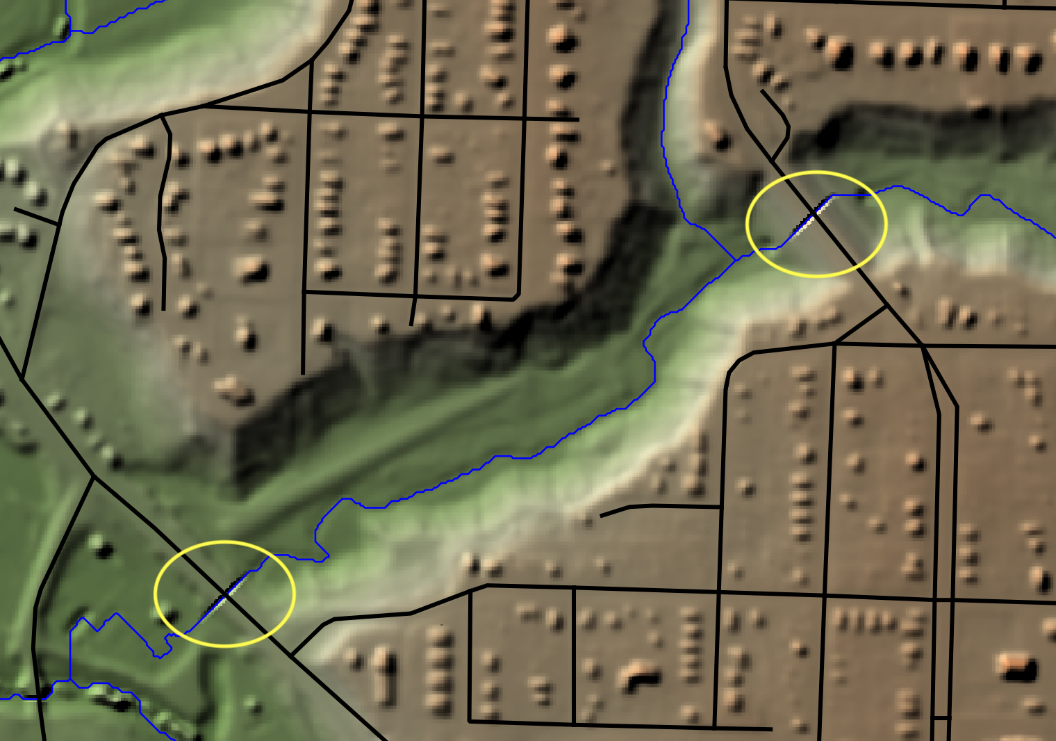
BurnStreamsAtRoads
This tool decrements (lowers) the elevations of pixels within an input digital elevation model (DEM) (--dem)
along an input vector stream network (--streams) at the sites of road (--roads) intersections. In addition
to the input data layers, the user must specify the output raster DEM (--output), and the maximum road embankment width
(--width), in map units. The road width parameter is used to determine the length of channel along stream
lines, at the junctions between streams and roads, that the burning (i.e. decrementing) operation occurs. The
algorithm works by identifying stream-road intersection cells, then traversing along the rasterized stream path
in the upstream and downstream directions by half the maximum road embankment width. The minimum elevation in each
stream traversal is identified and then elevations that are higher than this value are lowered to the minimum
elevation during a second stream traversal.
Reference:
Lindsay JB. 2016. The practice of DEM stream burning revisited. Earth Surface Processes and Landforms, 41(5): 658–668. DOI: 10.1002/esp.3888
See Also: RasterStreamsToVector, RasterizeStreams
Parameters:
| Flag | Description |
|---|---|
| --dem | Input raster digital elevation model (DEM) file |
| --streams | Input vector streams file |
| --roads | Input vector roads file |
| -o, --output | Output raster file |
| --width | Maximum road embankment width, in map units |
Python function:
wbt.burn_streams_at_roads(
    dem,
    streams,
    roads,
    output,
    width=None,
    callback=default_callback
)
Command-line Interface:
>>./whitebox_tools -r=BurnStreamsAtRoads -v ^
--wd="/path/to/data/" --dem=raster.tif --streams=streams.shp ^
--roads=roads.shp -o=output.tif --width=50.0
Author: Dr. John Lindsay
Created: 30/10/2019
Last Modified: 29/12/2019
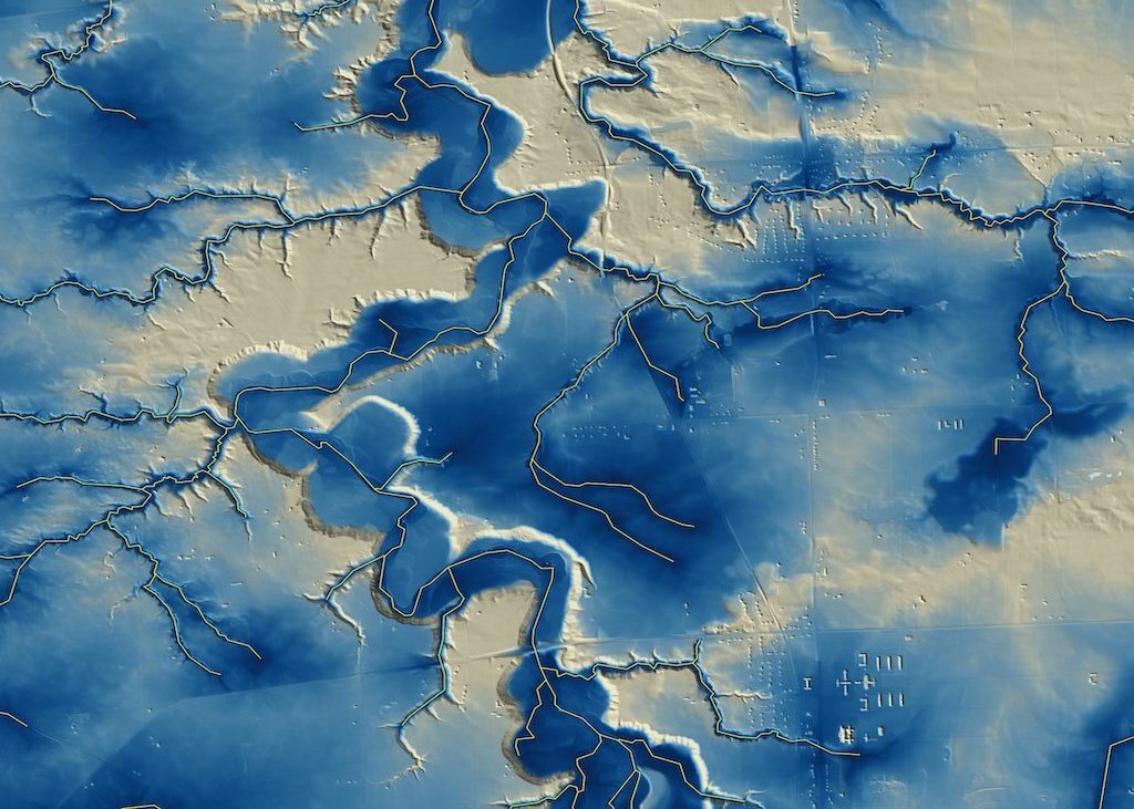
D8FlowAccumulation
This tool is used to generate a flow accumulation grid (i.e. catchment area) using the
D8 (O'Callaghan and Mark, 1984) algorithm. This algorithm is an example of single-flow-direction
(SFD) method because the flow entering each grid cell is routed to only one downslope neighbour,
i.e. flow divergence is not permitted. The user must specify the name of the input digital
elevation model (DEM) or flow pointer raster (--input) derived using the D8 or Rho8 method
(D8Pointer, Rho8Pointer). If an input DEM is used, it must have
been hydrologically corrected to remove all spurious depressions and flat areas. DEM pre-processing
is usually achieved using the BreachDepressionsLeastCost or FillDepressions tools. If a D8 pointer
raster is input, the user must also specify the optional --pntr flag. If the D8 pointer follows
the Esri pointer scheme, rather than the default WhiteboxTools scheme, the user must also specify the
optional --esri_pntr flag.
In addition to the input DEM/pointer, the user must specify the output type. The output flow-accumulation
can be 1) cells (i.e. the number of inflowing grid cells), catchment area (i.e. the upslope area),
or specific contributing area (i.e. the catchment area divided by the flow width. The default value
is cells. The user must also specify whether the output flow-accumulation grid should be
log-tranformed (--log), i.e. the output, if this option is selected, will be the natural-logarithm of the
accumulated flow value. This is a transformation that is often performed to better visualize the
contributing area distribution. Because contributing areas tend to be very high along valley bottoms
and relatively low on hillslopes, when a flow-accumulation image is displayed, the distribution of
values on hillslopes tends to be 'washed out' because the palette is stretched out to represent the
highest values. Log-transformation provides a means of compensating for this phenomenon. Importantly,
however, log-transformed flow-accumulation grids must not be used to estimate other secondary terrain
indices, such as the wetness index, or relative stream power index.
Grid cells possessing the NoData value in the input DEM/pointer raster are assigned the NoData value in the output flow-accumulation image.
Reference:
O'Callaghan, J. F., & Mark, D. M. 1984. The extraction of drainage networks from digital elevation data. Computer Vision, Graphics, and Image Processing, 28(3), 323-344.
See Also: FD8FlowAccumulation, QuinnFlowAccumulation, QinFlowAccumulation, DInfFlowAccumulation, MDInfFlowAccumulation, Rho8Pointer, D8Pointer, BreachDepressionsLeastCost, FillDepressions
Parameters:
| Flag | Description |
|---|---|
| -i, --input | Input raster DEM or D8 pointer file |
| -o, --output | Output raster file |
| --out_type | Output type; one of 'cells' (default), 'catchment area', and 'specific contributing area' |
| --log | Optional flag to request the output be log-transformed |
| --clip | Optional flag to request clipping the display max by 1% |
| --pntr | Is the input raster a D8 flow pointer rather than a DEM? |
| --esri_pntr | Input D8 pointer uses the ESRI style scheme |
Python function:
wbt.d8_flow_accumulation(
    i,
    output,
    out_type="cells",
    log=False,
    clip=False,
    pntr=False,
    esri_pntr=False,
    callback=default_callback
)
Command-line Interface:
>>./whitebox_tools -r=D8FlowAccumulation -v ^
--wd="/path/to/data/" --input=DEM.tif -o=output.tif ^
--out_type='cells'
>>./whitebox_tools -r=D8FlowAccumulation -v ^
--wd="/path/to/data/" --input=DEM.tif -o=output.tif ^
--out_type='specific catchment area' --log --clip
Author: Dr. John Lindsay
Created: 26/016/2017
Last Modified: 29/08/2021
D8MassFlux
This tool can be used to perform a mass flux calculation using DEM-based surface flow-routing techniques.
For example, it could be used to model the distribution of sediment or phosphorous within a catchment.
Flow-routing is based on a D8 flow pointer (i.e. flow direction) derived from an input depresionless DEM
(--dem). The user must also specify the names of loading (--loading), efficiency (--efficiency), and
absorption (--absorption) rasters, as well as the output raster. Mass Flux operates very much like a
flow-accumulation operation except that rather than accumulating catchment areas the algorithm routes a
quantity of mass, the spatial distribution of which is specified within the loading image. The efficiency and
absorption rasters represent spatial distributions of losses to the accumulation process, the difference
being that the efficiency raster is a proportional loss (e.g. only 50% of material within a particular grid
cell will be directed downslope) and the absorption raster is an loss specified as a quantity in the same
units as the loading image. The efficiency image can range from 0 to 1, or alternatively, can be expressed as
a percentage. The equation for determining the mass sent from one grid cell to a neighbouring grid cell is:
Outflowing Mass = (Loading - Absorption + Inflowing Mass) × Efficiency
This tool assumes that each of the three input rasters have the same number of rows and columns and that any NoData cells present are the same among each of the inputs.
See Also: DInfMassFlux
Parameters:
| Flag | Description |
|---|---|
| --dem | Input raster DEM file |
| --loading | Input loading raster file |
| --efficiency | Input efficiency raster file |
| --absorption | Input absorption raster file |
| -o, --output | Output raster file |
Python function:
wbt.d8_mass_flux(
    dem,
    loading,
    efficiency,
    absorption,
    output,
    callback=default_callback
)
Command-line Interface:
>>./whitebox_tools -r=D8MassFlux -v --wd="/path/to/data/" ^
--dem=DEM.tif --loading=load.tif --efficiency=eff.tif ^
--absorption=abs.tif -o=output.tif
Author: Dr. John Lindsay
Created: Dec. 29, 2017
Last Modified: 12/10/2018
D8Pointer
This tool is used to generate a flow pointer grid using the simple D8 (O'Callaghan and Mark, 1984) algorithm. The
user must specify the name (--dem) of a digital elevation model (DEM) that has been hydrologically
corrected to remove all spurious depressions and flat areas. DEM pre-processing is usually achieved using
either the BreachDepressions or FillDepressions tool. The local drainage direction raster output (--output)
by this tool serves as a necessary input for several other spatial hydrology and stream network analysis tools
in the toolset. Some tools will calculate this flow pointer raster directly from the input DEM.
By default, D8 flow pointers use the following clockwise, base-2 numeric index convention:
| . | . | . |
|---|---|---|
| 64 | 128 | 1 |
| 32 | 0 | 2 |
| 16 | 8 | 4 |
Notice that grid cells that have no lower neighbours are assigned a flow direction of zero. In a DEM that has been
pre-processed to remove all depressions and flat areas, this condition will only occur along the edges of the grid.
If the pointer file contains ESRI flow direction values instead, the --esri_pntr parameter must be specified.
Grid cells possessing the NoData value in the input DEM are assigned the NoData value in the output image.
Memory Usage
The peak memory usage of this tool is approximately 10 bytes per grid cell.
Reference:
O'Callaghan, J. F., & Mark, D. M. (1984). The extraction of drainage networks from digital elevation data. Computer vision, graphics, and image processing, 28(3), 323-344.
See Also: DInfPointer, FD8Pointer, BreachDepressions, FillDepressions
Parameters:
| Flag | Description |
|---|---|
| -i, --dem | Input raster DEM file |
| -o, --output | Output raster file |
| --esri_pntr | D8 pointer uses the ESRI style scheme |
Python function:
wbt.d8_pointer(
    dem,
    output,
    esri_pntr=False,
    callback=default_callback
)
Command-line Interface:
>>./whitebox_tools -r=D8Pointer -v --wd="/path/to/data/" ^
--dem=DEM.tif -o=output.tif
Author: Dr. John Lindsay
Created: 16/06/2017
Last Modified: 18/10/2019
DInfFlowAccumulation
This tool is used to generate a flow accumulation grid (i.e. contributing area) using the D-infinity algorithm
(Tarboton, 1997). This algorithm is an examples of a multiple-flow-direction (MFD) method because the flow entering
each grid cell is routed to one or two downslope neighbour, i.e. flow divergence is permitted. The user must
specify the name of the input digital elevation model or D-infinity pointer raster (--input). If an input DEM is
specified, the DEM should have been hydrologically corrected
to remove all spurious depressions and flat areas. DEM pre-processing is usually achieved using the
BreachDepressionsLeastCost or FillDepressions tool.
In addition to the input DEM/pointer raster name, the user must specify the output type (--out_type). The output
flow-accumulation
can be 1) specific catchment area (SCA), which is the upslope contributing area divided by the contour length (taken
as the grid resolution), 2) total catchment area in square-metres, or 3) the number of upslope grid cells. The user
must also specify whether the output flow-accumulation grid should be log-tranformed, i.e. the output, if this option
is selected, will be the natural-logarithm of the accumulated area. This is a transformation that is often performed
to better visualize the contributing area distribution. Because contributing areas tend to be very high along valley
bottoms and relatively low on hillslopes, when a flow-accumulation image is displayed, the distribution of values on
hillslopes tends to be 'washed out' because the palette is stretched out to represent the highest values.
Log-transformation (--log) provides a means of compensating for this phenomenon. Importantly, however, log-transformed
flow-accumulation grids must not be used to estimate other secondary terrain indices, such as the wetness index, or
relative stream power index.
Grid cells possessing the NoData value in the input DEM/pointer raster are assigned the NoData value in the output flow-accumulation image. The output raster is of the float data type and continuous data scale.
Reference:
Tarboton, D. G. (1997). A new method for the determination of flow directions and upslope areas in grid digital elevation models. Water resources research, 33(2), 309-319.
See Also:
DInfPointer, D8FlowAccumulation, QuinnFlowAccumulation, QinFlowAccumulation, FD8FlowAccumulation, MDInfFlowAccumulation, Rho8Pointer`, BreachDepressionsLeastCost, FillDepressions
Parameters:
| Flag | Description |
|---|---|
| -i, --input | Input raster DEM or D-infinity pointer file |
| -o, --output | Output raster file |
| --out_type | Output type; one of 'cells', 'sca' (default), and 'ca' |
| --threshold | Optional convergence threshold parameter, in grid cells; default is infinity |
| --log | Optional flag to request the output be log-transformed |
| --clip | Optional flag to request clipping the display max by 1% |
| --pntr | Is the input raster a D-infinity flow pointer rather than a DEM? |
Python function:
wbt.d_inf_flow_accumulation(
    i,
    output,
    out_type="Specific Contributing Area",
    threshold=None,
    log=False,
    clip=False,
    pntr=False,
    callback=default_callback
)
Command-line Interface:
>>./whitebox_tools -r=DInfFlowAccumulation -v ^
--wd="/path/to/data/" --input=DEM.tif -o=output.tif ^
--out_type=sca
>>./whitebox_tools -r=DInfFlowAccumulation -v ^
--wd="/path/to/data/" --input=DEM.tif -o=output.tif ^
--out_type=sca --threshold=10000 --log --clip
Author: Dr. John Lindsay
Created: 24/06/2017
Last Modified: 21/02/2020
DInfMassFlux
This tool can be used to perform a mass flux calculation using DEM-based surface flow-routing techniques. For
example, it could be used to model the distribution of sediment or phosphorous within a catchment. Flow-routing
is based on a D-Infinity flow pointer derived from an input DEM (--dem). The user must also specify the
names of loading (--loading), efficiency (--efficiency), and absorption (--absorption) rasters, as well
as the output raster. Mass Flux operates very much like a flow-accumulation operation except that rather than
accumulating catchment areas the algorithm routes a quantity of mass, the spatial distribution of which is
specified within the loading image. The efficiency and absorption rasters represent spatial distributions of
losses to the accumulation process, the difference being that the efficiency raster is a proportional loss (e.g.
only 50% of material within a particular grid cell will be directed downslope) and the absorption raster is an
loss specified as a quantity in the same units as the loading image. The efficiency image can range from 0 to 1,
or alternatively, can be expressed as a percentage. The equation for determining the mass sent from one grid cell
to a neighbouring grid cell is:
Outflowing Mass = (Loading - Absorption + Inflowing Mass) × Efficiency
This tool assumes that each of the three input rasters have the same number of rows and columns and that any NoData cells present are the same among each of the inputs.
See Also: D8MassFlux
Parameters:
| Flag | Description |
|---|---|
| --dem | Input raster DEM file |
| --loading | Input loading raster file |
| --efficiency | Input efficiency raster file |
| --absorption | Input absorption raster file |
| -o, --output | Output raster file |
Python function:
wbt.d_inf_mass_flux(
    dem,
    loading,
    efficiency,
    absorption,
    output,
    callback=default_callback
)
Command-line Interface:
>>./whitebox_tools -r=DInfMassFlux -v --wd="/path/to/data/" ^
--dem=DEM.tif --loading=load.tif --efficiency=eff.tif ^
--absorption=abs.tif -o=output.tif
Author: Dr. John Lindsay
Created: Dec. 29, 2017
Last Modified: 12/10/2018
DInfPointer
This tool is used to generate a flow pointer grid (i.e. flow direction) using the D-infinity
(Tarboton, 1997) algorithm. Dinf is a multiple-flow-direction (MFD) method because the flow
entering each grid cell is routed one or two downslope neighbours, i.e. flow divergence is permitted.
The user must specify the name of a digital elevation model (DEM; --dem) that has been hydrologically
corrected to remove all spurious depressions and flat areas (BreachDepressions, FillDepressions).
DEM pre-processing is usually achieved using the BreachDepressions or FillDepressions tool1. Flow
directions are specified in the output flow-pointer grid (--output) as azimuth degrees measured from
north, i.e. any value between 0 and 360 degrees is possible. A pointer value of -1 is used to designate
a grid cell with no flow-pointer. This occurs when a grid cell has no downslope neighbour, i.e. a pit
cell or topographic depression. Like aspect grids, Dinf flow-pointer grids are best visualized using
a circular greyscale palette.
Grid cells possessing the NoData value in the input DEM are assigned the NoData value in the output image. The output raster is of the float data type and continuous data scale.
Reference:
Tarboton, D. G. (1997). A new method for the determination of flow directions and upslope areas in grid digital elevation models. Water resources research, 33(2), 309-319.
See Also: DInfFlowAccumulation, BreachDepressions, FillDepressions
Parameters:
| Flag | Description |
|---|---|
| -i, --dem | Input raster DEM file |
| -o, --output | Output raster file |
Python function:
wbt.d_inf_pointer(
    dem,
    output,
    callback=default_callback
)
Command-line Interface:
>>./whitebox_tools -r=DInfPointer -v --wd="/path/to/data/" ^
--dem=DEM.tif
Author: Dr. John Lindsay
Created: 26/06/2017
Last Modified: 13/02/2020
DepthInSink
This tool measures the depth that each grid cell in an input (--dem) raster digital elevation model (DEM)
lies within a sink feature, i.e. a closed topographic depression. A sink, or depression, is a bowl-like
landscape feature, which is characterized by interior drainage and groundwater recharge. The DepthInSink tool
operates by differencing a filled DEM, using the same depression filling method as FillDepressions, and the
original surface model.
In addition to the names of the input DEM (--dem) and the output raster (--output), the user must specify
whether the background value (i.e. the value assigned to grid cells that are not contained within sinks) should be
set to 0.0 (--zero_background) Without this optional parameter specified, the tool will use the NoData value
as the background value.
Reference:
Antonić, O., Hatic, D., & Pernar, R. (2001). DEM-based depth in sink as an environmental estimator. Ecological Modelling, 138(1-3), 247-254.
See Also: FillDepressions
Parameters:
| Flag | Description |
|---|---|
| -i, --dem | Input raster DEM file |
| -o, --output | Output raster file |
| --zero_background | Flag indicating whether the background value of zero should be used |
Python function:
wbt.depth_in_sink(
    dem,
    output,
    zero_background=False,
    callback=default_callback
)
Command-line Interface:
>>./whitebox_tools -r=DepthInSink -v --wd="/path/to/data/" ^
--dem=DEM.tif -o=output.tif --zero_background
Author: Dr. John Lindsay
Created: 11/07/2017
Last Modified: 05/12/2019
DepthToWater
Note this tool is part of a WhiteboxTools extension product. Please visit Whitebox Geospatial Inc. for information about purchasing a license activation key (https://www.whiteboxgeo.com/extension-pricing/).
This tool calculates the cartographic depth-to-water (DTW) index described by Murphy et al. (2009). The DTW index has been shown to be related to soil moisture, and is useful for identifying low-lying positions that are likely to experience surface saturated conditions. In this regard, it is similar to each of WetnessIndex, ElevationAboveStream (HAND), and probability-of-depressions (i.e. StochasticDepressionAnalysis).
The index is the cumulative slope gradient along the least-slope path connecting each grid cell in an input DEM (--dem) to
a surface water cell. Tangent slope (i.e. rise / run) is calculated for each grid cell based on the neighbouring elevation
values in the input DEM. The algorithm
operates much like a cost-accumulation analysis (CostDistance), where the cost of moving through a cell is determined
by the cell's tangent slope value and the distance travelled. Therefore, lower DTW values are associated with wetter soils and
higher values indicate drier conditions, over longer time periods. Areas of surface water have DTW values of zero. The user
must input surface water features, including vector stream lines (--streams) and/or vector waterbody polygons
(--lakes, i.e. lakes, ponds, wetlands, etc.). At least one of these two optional water feature inputs must be specified. The
tool internally rasterizes these vector features, setting the DTW value in the output raster to zero. DTW tends
to increase with greater distances from surface water features, and increases more slowly in flatter topography and more
rapidly in steeper settings. Murphy et al. (2009) state that DTW is a probablistic model that assumes uniform soil properties,
climate, and vegetation.
Note that DTW values are highly dependent upon the accuracy and extent of the input streams/lakes layer(s).
References:
Murphy, PNC, Gilvie, JO, and Arp, PA (2009) Topographic modelling of soil moisture conditions: a comparison and verification of two models. European Journal of Soil Science, 60, 94–109, DOI: 10.1111/j.1365-2389.2008.01094.x.
See Also: WetnessIndex, ElevationAboveStream, StochasticDepressionAnalysis
Parameters:
| Flag | Description |
|---|---|
| --dem | Name of the input raster DEM file |
| --streams | Name of the input streams vector (optional) |
| --lakes | Name of the input lakes vector (optional) |
| -o, --output | Name of the output raster image file |
Python function:
wbt.depth_to_water(
    dem,
    output,
    streams=None,
    lakes=None,
    callback=default_callback
)
Command-line Interface:
>> ./whitebox_tools -r=DepthToWater --dem=DEM.tif ^
--streams=streams.shp --lakes=waterbodies.shp -o=output.tif
Source code is unavailable due to proprietary license.
Author: Whitebox Geospatial Inc. (c)
Created: 24/05/2022
Last Modified: 24/05/2022
DownslopeDistanceToStream
This tool can be used to calculate the distance from each grid cell in a raster to the nearest stream cell,
measured along the downslope flowpath. The user must specify the name of an input digital elevation model (--dem)
and streams raster (--streams). The DEM must have been pre-processed to remove artifact topographic depressions
and flat areas (see BreachDepressions). The streams raster should have been created using one of the DEM-based
stream mapping methods, i.e. contributing area thresholding. Stream cells are designated in this raster as all
non-zero values. The output of this tool, along with the ElevationAboveStream tool, can be useful for preliminary
flood plain mapping when combined with high-accuracy DEM data.
By default, this tool calculates flow-path using the D8 flow algorithm. However, the user may specify (--dinf) that
the tool should use the D-infinity algorithm instead.
See Also: ElevationAboveStream, DistanceToOutlet
Parameters:
| Flag | Description |
|---|---|
| -i, --dem | Input raster DEM file |
| --streams | Input raster streams file |
| -o, --output | Output raster file |
| --dinf | Use the D-infinity flow algorithm instead of D8? |
Python function:
wbt.downslope_distance_to_stream(
    dem,
    streams,
    output,
    dinf=False,
    callback=default_callback
)
Command-line Interface:
>>./whitebox_tools -r=DownslopeDistanceToStream -v ^
--wd="/path/to/data/" --dem='dem.tif' --streams='streams.tif' ^
-o='output.tif'
Author: Dr. John Lindsay
Created: 9/07/2017
Last Modified: 04/10/2019
DownslopeFlowpathLength
This tool can be used to calculate the downslope flowpath length from each grid cell in a raster to
an outlet cell either at the edge of the grid or at the outlet point of a watershed. The user must
specify the name of a flow pointer grid (--d8_pntr) derived using the D8 flow algorithm (D8Pointer).
This grid should be derived from a digital elevation model (DEM) that has been pre-processed to remove
artifact topographic depressions and flat areas (BreachDepressions, FillDepressions). The user may also
optionally provide watershed (--watersheds) and weights (--weights) images. The optional watershed
image can be used to define one or more irregular-shaped watershed boundaries. Flowpath lengths are
measured within each watershed in the watershed image (each defined by a unique identifying number) as
the flowpath length to the watershed's outlet cell.
The optional weight image is multiplied by the flow-length through each grid cell. This can be useful when there is a need to convert the units of the output image. For example, the default unit of flowpath lengths is the same as the input image(s). Thus, if the input image has X-Y coordinates measured in metres, the output image will likely contain very large values. A weight image containing a value of 0.001 for each grid cell will effectively convert the output flowpath lengths into kilometres. The weight image can also be used to convert the flowpath distances into travel times by multiplying the flow distance through a grid cell by the average velocity.
NoData valued grid cells in any of the input images will be assigned NoData values in the output image. The output raster is of the float data type and continuous data scale.
See Also: D8Pointer, ElevationAboveStream, BreachDepressions, FillDepressions, Watershed
Parameters:
| Flag | Description |
|---|---|
| --d8_pntr | Input D8 pointer raster file |
| --watersheds | Optional input watershed raster file |
| --weights | Optional input weights raster file |
| -o, --output | Output raster file |
| --esri_pntr | D8 pointer uses the ESRI style scheme |
Python function:
wbt.downslope_flowpath_length(
    d8_pntr,
    output,
    watersheds=None,
    weights=None,
    esri_pntr=False,
    callback=default_callback
)
Command-line Interface:
>>./whitebox_tools -r=DownslopeFlowpathLength -v ^
--wd="/path/to/data/" --d8_pntr=pointer.tif ^
-o=flowpath_len.tif
>>./whitebox_tools ^
-r=DownslopeFlowpathLength -v --wd="/path/to/data/" ^
--d8_pntr=pointer.tif --watersheds=basin.tif ^
--weights=weights.tif -o=flowpath_len.tif --esri_pntr
Author: Dr. John Lindsay
Created: 08/07/2017
Last Modified: 18/10/2019
EdgeContamination
This tool identifs grid cells in a DEM for which the upslope area extends beyond the raster data extent, so-called 'edge-contamined cells'. If a significant number of edge contaminated cells intersect with your area of interest, it is likely that any estimate of upslope area (i.e. flow accumulation) will be under-estimated.
The user must specify the name (--dem) of the input digital elevation model (DEM) and the
output file (--output). The DEM must have been hydrologically corrected to remove all spurious depressions and
flat areas. DEM pre-processing is usually achieved using either the BreachDepressions (also BreachDepressionsLeastCost)
or FillDepressions tool.
Additionally, the user must specify the type of flow algorithm used for the analysis (-flow_type), which must be
one of 'd8', 'mfd', or 'dinf', based on each of the D8FlowAccumulation, FD8FlowAccumulation, DInfFlowAccumulation
methods respectively.
See Also: D8FlowAccumulation, FD8FlowAccumulation, DInfFlowAccumulation
Parameters:
| Flag | Description |
|---|---|
| -d, --dem | Name of the input DEM raster file; must be depressionless |
| -o, --output | Name of the output raster file |
| --flow_type | Flow algorithm type, one of 'd8', 'mfd', or 'dinf' |
| --zfactor | Optional multiplier for when the vertical and horizontal units are not the same |
Python function:
wbt.edge_contamination(
    dem,
    output,
    flow_type="mfd",
    zfactor="",
    callback=default_callback
)
Command-line Interface:
-./whitebox_tools -r=EdgeContamination --dem=DEM.tif ^
--output=edge_cont.tif --flow_type='dinf'
Author: Dr. John Lindsay
Created: 23/07/2021
Last Modified: 23/07/2021
ElevationAboveStream
This tool can be used to calculate the elevation of each grid cell in a raster above the nearest stream cell,
measured along the downslope flowpath. This terrain index, a measure of relative topographic position, is
essentially equivalent to the 'height above drainage' (HAND), as described by Renno et al. (2008). The user must
specify the name of an input digital elevation model (--dem) and streams raster (--streams). The DEM
must have been pre-processed to remove artifact topographic depressions and flat areas (see BreachDepressions).
The streams raster should have been created using one of the DEM-based stream mapping methods, i.e. contributing
area thresholding. Stream cells are designated in this raster as all non-zero values. The output of this tool,
along with the DownslopeDistanceToStream tool, can be useful for preliminary flood plain mapping when combined
with high-accuracy DEM data.
The difference between ElevationAboveStream and ElevationAboveStreamEuclidean is that the former calculates distances along drainage flow-paths while the latter calculates straight-line distances to streams channels.
Reference:
Renno, C. D., Nobre, A. D., Cuartas, L. A., Soares, J. V., Hodnett, M. G., Tomasella, J., & Waterloo, M. J. (2008). HAND, a new terrain descriptor using SRTM-DEM: Mapping terra-firme rainforest environments in Amazonia. Remote Sensing of Environment, 112(9), 3469-3481.
See Also: ElevationAboveStreamEuclidean, DownslopeDistanceToStream, ElevAbovePit, BreachDepressions
Parameters:
| Flag | Description |
|---|---|
| -i, --dem | Input raster DEM file |
| --streams | Input raster streams file |
| -o, --output | Output raster file |
Python function:
wbt.elevation_above_stream(
    dem,
    streams,
    output,
    callback=default_callback
)
Command-line Interface:
>>./whitebox_tools -r=ElevationAboveStream -v ^
--wd="/path/to/data/" --dem='dem.tif' --streams='streams.tif' ^
-o='output.tif'
Author: Dr. John Lindsay
Created: July 9, 2017
Last Modified: 12/10/2018
ElevationAboveStreamEuclidean
This tool can be used to calculate the elevation of each grid cell in a raster above the nearest stream cell,
measured along the straight-line distance. This terrain index, a measure of relative topographic position, is
related to the 'height above drainage' (HAND), as described by Renno et al. (2008). HAND is generally estimated
with distances measured along drainage flow-paths, which can be calculated using the ElevationAboveStream tool.
The user must specify the name of an input digital elevation model (--dem) and streams raster (--streams).
Stream cells are designated in this raster as all non-zero values. The output of this tool,
along with the DownslopeDistanceToStream tool, can be useful for preliminary flood plain mapping when combined
with high-accuracy DEM data.
The difference between ElevationAboveStream and ElevationAboveStreamEuclidean is that the former calculates distances along drainage flow-paths while the latter calculates straight-line distances to streams channels.
Reference:
Renno, C. D., Nobre, A. D., Cuartas, L. A., Soares, J. V., Hodnett, M. G., Tomasella, J., & Waterloo, M. J. (2008). HAND, a new terrain descriptor using SRTM-DEM: Mapping terra-firme rainforest environments in Amazonia. Remote Sensing of Environment, 112(9), 3469-3481.
See Also: ElevationAboveStream, DownslopeDistanceToStream, ElevAbovePit
Parameters:
| Flag | Description |
|---|---|
| -i, --dem | Input raster DEM file |
| --streams | Input raster streams file |
| -o, --output | Output raster file |
Python function:
wbt.elevation_above_stream_euclidean(
    dem,
    streams,
    output,
    callback=default_callback
)
Command-line Interface:
>>./whitebox_tools -r=ElevationAboveStreamEuclidean -v ^
--wd="/path/to/data/" -i=DEM.tif --streams=streams.tif ^
-o=output.tif
Author: Dr. John Lindsay
Created: 11/03/2018
Last Modified: 12/10/2018
Fd8FlowAccumulation
This tool is used to generate a flow accumulation grid (i.e. contributing area) using the FD8 algorithm (Freeman,
1991), sometimes referred to as FMFD. This algorithm is an examples of a multiple-flow-direction (MFD) method because the flow entering each
grid cell is routed to each downslope neighbour, i.e. flow divergence is permitted. The user must specify the
name (--dem) of the input digital elevation model (DEM). The DEM must have been hydrologically
corrected to remove all spurious depressions and flat areas. DEM pre-processing is usually achieved using
either the BreachDepressions (also BreachDepressionsLeastCost) or FillDepressions tool. A value must also be specified for the exponent parameter
(--exponent), a number that controls the degree of dispersion in the resulting flow-accumulation grid. A lower
value yields greater apparent flow dispersion across divergent hillslopes. Some experimentation suggests that a
value of 1.1 is appropriate (Freeman, 1991), although this is almost certainly landscape-dependent.
In addition to the input DEM, the user must specify the output type (--out_type). The output flow-accumulation
can be 1) cells (i.e. the number of inflowing grid cells), catchment area (i.e. the upslope area),
or specific contributing area (i.e. the catchment area divided by the flow width. The default value
is cells. The user must also specify whether the output flow-accumulation grid should be
log-tranformed (--log), i.e. the output, if this option is selected, will be the natural-logarithm of the
accumulated flow value. This is a transformation that is often performed to better visualize the
contributing area distribution. Because contributing areas tend to be very high along valley bottoms
and relatively low on hillslopes, when a flow-accumulation image is displayed, the distribution of
values on hillslopes tends to be 'washed out' because the palette is stretched out to represent the
highest values. Log-transformation provides a means of compensating for this phenomenon. Importantly,
however, log-transformed flow-accumulation grids must not be used to estimate other secondary terrain
indices, such as the wetness index, or relative stream power index.
The non-dispersive threshold (--threshold) is a flow-accumulation value (measured in upslope grid cells,
which is directly proportional to area) above which flow dispersion is no longer permitted. Grid cells with
flow-accumulation values above this threshold will have their flow routed in a manner that is similar to
the D8 single-flow-direction algorithm, directing all flow towards the steepest downslope neighbour. This
is usually done under the assumption that flow dispersion, whilst appropriate on hillslope areas, is not
realistic once flow becomes channelized.
Reference:
Freeman, T. G. (1991). Calculating catchment area with divergent flow based on a regular grid. Computers and Geosciences, 17(3), 413-422.
See Also: D8FlowAccumulation, QuinnFlowAccumulation, QinFlowAccumulation, DInfFlowAccumulation, MDInfFlowAccumulation, Rho8Pointer
Parameters:
| Flag | Description |
|---|---|
| -i, --dem | Input raster DEM file |
| -o, --output | Output raster file |
| --out_type | Output type; one of 'cells', 'specific contributing area' (default), and 'catchment area' |
| --exponent | Optional exponent parameter; default is 1.1 |
| --threshold | Optional convergence threshold parameter, in grid cells; default is infinity |
| --log | Optional flag to request the output be log-transformed |
| --clip | Optional flag to request clipping the display max by 1% |
Python function:
wbt.fd8_flow_accumulation(
    dem,
    output,
    out_type="specific contributing area",
    exponent=1.1,
    threshold=None,
    log=False,
    clip=False,
    callback=default_callback
)
Command-line Interface:
>>./whitebox_tools -r=FD8FlowAccumulation -v ^
--wd="/path/to/data/" --dem=DEM.tif -o=output.tif ^
--out_type='cells'
>>./whitebox_tools -r=FD8FlowAccumulation -v ^
--wd="/path/to/data/" --dem=DEM.tif -o=output.tif ^
--out_type='catchment area' --exponent=1.5 --threshold=10000 ^
--log --clip
Author: Dr. John Lindsay
Created: 26/06/2017
Last Modified: 15/07/2021
Fd8Pointer
This tool is used to generate a flow pointer grid (i.e. flow direction) using the FD8 (Freeman, 1991) algorithm.
FD8 is a multiple-flow-direction (MFD) method because the flow entering each grid cell is routed one or more
downslope neighbours, i.e. flow divergence is permitted. The user must specify the name of a digital elevation model
(DEM; --dem) that has been hydrologically corrected to remove all spurious depressions and flat areas.
DEM pre-processing is usually achieved using the BreachDepressions or FillDepressions tools.
By default, D8 flow pointers use the following clockwise, base-2 numeric index convention:
| . | . | . |
|---|---|---|
| 64 | 128 | 1 |
| 32 | 0 | 2 |
| 16 | 8 | 4 |
In the case of the FD8 algorithm, some portion of the flow entering a grid cell will be sent to each downslope neighbour. Thus, the FD8 flow-pointer value is the sum of each of the individual pointers for all downslope neighbours. For example, if a grid cell has downslope neighbours to the northeast, east, and south the corresponding FD8 flow-pointer value will be 1 + 2 + 8 = 11. Using the naming convention above, this is the only combination of flow-pointers that will result in the combined value of 11. Using the base-2 naming convention allows for the storage of complex combinations of flow-points using a single numeric value, which is the reason for using this somewhat odd convention.
Reference:
Freeman, T. G. (1991). Calculating catchment area with divergent flow based on a regular grid. Computers and Geosciences, 17(3), 413-422.
See Also: FD8FlowAccumulation, D8Pointer, DInfPointer, BreachDepressions, FillDepressions
Parameters:
| Flag | Description |
|---|---|
| -i, --dem | Input raster DEM file |
| -o, --output | Output raster file |
Python function:
wbt.fd8_pointer(
    dem,
    output,
    callback=default_callback
)
Command-line Interface:
>>./whitebox_tools -r=FD8Pointer -v --wd="/path/to/data/" ^
--dem=DEM.tif -o=output.tif
Author: Dr. John Lindsay
Created: 28/06/2017
Last Modified: 12/10/2018
FillBurn
Burns streams into a digital elevation model (DEM) using the FillBurn (Saunders, 1999) method which produces a hydro-enforced DEM. This tool uses the algorithm described in:
Lindsay JB. 2016. The practice of DEM stream burning revisited. Earth Surface Processes and Landforms, 41(5): 658-668. DOI: 10.1002/esp.3888
And:
Saunders, W. 1999. Preparation of DEMs for use in environmental modeling analysis, in: ESRI User Conference. pp. 24-30.
The TopologicalBreachBurn tool, contained within the Whitebox Toolset Extension (WTE), should be preferred to this FillBurn, because it accounts for the topological errors that frequently occur when burning vector streams into a DEM.
See Also: TopologicalBreachBurn, PruneVectorStreams
Parameters:
| Flag | Description |
|---|---|
| --dem | Input raster DEM file |
| --streams | Input vector streams file |
| -o, --output | Output raster file |
Python function:
wbt.fill_burn(
    dem,
    streams,
    output,
    callback=default_callback
)
Command-line Interface:
>>./whitebox_tools -r=FillBurn -v --wd="/path/to/data/" ^
--dem=DEM.tif --streams=streams.shp -o=dem_burned.tif
Author: Dr. John Lindsay
Created: 01/04/2018
Last Modified: 22/10/2019
FillDepressions
This tool can be used to fill all of the depressions in a digital elevation model (DEM) and to remove the
flat areas. This is a common pre-processing step required by many flow-path analysis tools to ensure continuous
flow from each grid cell to an outlet located along the grid edge. The FillDepressions algorithm operates
by first identifying single-cell pits, that is, interior grid cells with no lower neighbouring cells. Each pit
cell is then visited from highest to lowest and a priority region-growing operation is initiated. The area of
monotonically increasing elevation, starting from the pit cell and growing based on flood order, is identified.
Once a cell, that has not been previously visited and possessing a lower elevation than its discovering neighbour
cell, is identified the discovering neighbour is labelled as an outlet (spill point) and the outlet elevation is
noted. The algorithm then back-fills the labelled region, raising the elevation in the output DEM (--output) to
that of the outlet. Once this process is completed for each pit cell (noting that nested pit cells are often
solved by prior pits) the flat regions of filled pits are optionally treated (--fix_flats) with an applied
small slope gradient away from outlets (note, more than one outlet cell may exist for each depression). The user
may optionally specify the size of the elevation increment used to solve flats (--flat_increment), although
it is best to not specify this optional value and to let the algorithm determine the most suitable value itself.
The flat-fixing method applies a small gradient away from outlets using another priority region-growing operation (i.e.
based on a priority queue operation), where priorities are set by the elevations in the input DEM (--input). This
in effect ensures a gradient away from outlet cells but also following the natural pre-conditioned topography internal
to depression areas. For example, if a large filled area occurs upstream of a damming road-embankment, the filled
DEM will possess flow directions that are similar to the un-flooded valley, with flow following the valley bottom.
In fact, the above case is better handled using the BreachDepressionsLeastCost tool, which would simply cut through
the road embankment at the likely site of a culvert. However, the flat-fixing method of FillDepressions does mean
that this common occurrence in LiDAR DEMs is less problematic.
The BreachDepressionsLeastCost, while slightly less efficient than either other hydrological preprocessing methods, often provides a lower impact solution to topographic depressions and should be preferred in most applications. In comparison with the BreachDepressionsLeastCost tool, the depression filling method often provides a less satisfactory, higher impact solution. It is advisable that users try the BreachDepressionsLeastCost tool to remove depressions from their DEMs before using FillDepressions. Nonetheless, there are applications for which full depression filling using the FillDepressions tool may be preferred.
Note that this tool will not fill in NoData regions within the DEM. It is advisable to remove such regions using the FillMissingData tool prior to application.
See Also: BreachDepressionsLeastCost, BreachDepressions, Sink, DepthInSink, FillMissingData
Parameters:
| Flag | Description |
|---|---|
| -i, --dem | Input raster DEM file |
| -o, --output | Output raster file |
| --fix_flats | Optional flag indicating whether flat areas should have a small gradient applied |
| --flat_increment | Optional elevation increment applied to flat areas |
| --max_depth | Optional maximum depression depth to fill |
Python function:
wbt.fill_depressions(
    dem,
    output,
    fix_flats=True,
    flat_increment=None,
    max_depth=None,
    callback=default_callback
)
Command-line Interface:
>>./whitebox_tools -r=FillDepressions -v ^
--wd="/path/to/data/" --dem=DEM.tif -o=output.tif ^
--fix_flats
Author: Dr. John Lindsay
Created: 28/06/2017
Last Modified: 12/12/2019
FillDepressionsPlanchonAndDarboux
This tool can be used to fill all of the depressions in a digital elevation model (DEM) and to remove the flat areas using the Planchon and Darboux (2002) method. This is a common pre-processing step required by many flow-path analysis tools to ensure continuous flow from each grid cell to an outlet located along the grid edge. This tool is currently not the most efficient depression-removal algorithm available in WhiteboxTools; FillDepressions and BreachDepressionsLeastCost are both more efficient and often produce better, lower-impact results.
The user may optionally specify the size of the elevation increment used to solve flats (--flat_increment), although
it is best not to specify this optional value and to let the algorithm determine the most suitable value itself.
Reference:
Planchon, O. and Darboux, F., 2002. A fast, simple and versatile algorithm to fill the depressions of digital elevation models. Catena, 46(2-3), pp.159-176.
See Also: FillDepressions, BreachDepressionsLeastCost
Parameters:
| Flag | Description |
|---|---|
| -i, --dem | Input raster DEM file |
| -o, --output | Output raster file |
| --fix_flats | Optional flag indicating whether flat areas should have a small gradient applied |
| --flat_increment | Optional elevation increment applied to flat areas |
Python function:
wbt.fill_depressions_planchon_and_darboux(
    dem,
    output,
    fix_flats=True,
    flat_increment=None,
    callback=default_callback
)
Command-line Interface:
>>./whitebox_tools -r=FillDepressionsPlanchonAndDarboux -v ^
--wd="/path/to/data/" --dem=DEM.tif -o=output.tif ^
--fix_flats
Author: Dr. John Lindsay
Created: 02/02/2020
Last Modified: 02/02/2020
FillDepressionsWangAndLiu
This tool can be used to fill all of the depressions in a digital elevation model (DEM) and to remove the flat areas. This is a common pre-processing step required by many flow-path analysis tools to ensure continuous flow from each grid cell to an outlet located along the grid edge. The FillDepressionsWangAndLiu algorithm is based on the computationally efficient approach of examining each cell based on its spill elevation, starting from the edge cells, and visiting cells from lowest order using a priority queue. As such, it is based on the algorithm first proposed by Wang and Liu (2006). However, it is currently not the most efficient depression-removal algorithm available in WhiteboxTools; FillDepressions and BreachDepressionsLeastCost are both more efficient and often produce better, lower-impact results.
If the input DEM has gaps, or missing-data holes, that contain NoData values, it is better to use the FillMissingData tool to repair these gaps. This tool will interpolate values across the gaps and produce a more natural-looking surface than the flat areas that are produced by depression filling. Importantly, the FillDepressions tool algorithm implementation assumes that there are no 'donut hole' NoData gaps within the area of valid data. Any NoData areas along the edge of the grid will simply be ignored and will remain NoData areas in the output image.
The user may optionally specify the size of the elevation increment used to solve flats (--flat_increment), although
it is best not to specify this optional value and to let the algorithm determine the most suitable value itself.
Reference:
Wang, L. and Liu, H. 2006. An efficient method for identifying and filling surface depressions in digital elevation models for hydrologic analysis and modelling. International Journal of Geographical Information Science, 20(2): 193-213.
See Also: FillDepressions, BreachDepressionsLeastCost, BreachDepressions, FillMissingData
Parameters:
| Flag | Description |
|---|---|
| -i, --dem | Input raster DEM file |
| -o, --output | Output raster file |
| --fix_flats | Optional flag indicating whether flat areas should have a small gradient applied |
| --flat_increment | Optional elevation increment applied to flat areas |
Python function:
wbt.fill_depressions_wang_and_liu(
    dem,
    output,
    fix_flats=True,
    flat_increment=None,
    callback=default_callback
)
Command-line Interface:
>>./whitebox_tools -r=FillDepressionsWangAndLiu -v ^
--wd="/path/to/data/" --dem=DEM.tif -o=output.tif ^
--fix_flats
Author: Dr. John Lindsay
Created: 28/06/2017
Last Modified: 05/12/2019
FillSingleCellPits
This tool can be used to remove pits from a digital elevation model (DEM). Pits are single grid cells with no downslope neighbours. They are important because they impede overland flow-paths. This tool will remove any pits in the input DEM that can be resolved by raising the elevation of the pit such that flow will continue past the pit cell to one of the downslope neighbours. Notice that this tool can be a useful pre-processing technique before running one of the more robust depression breaching (BreachDepressions) or filling (FillDepressions) techniques, which are designed to remove larger depression features.
See Also: BreachDepressions, FillDepressions, BreachSingleCellPits
Parameters:
| Flag | Description |
|---|---|
| -i, --dem | Input raster DEM file |
| -o, --output | Output raster file |
Python function:
wbt.fill_single_cell_pits(
    dem,
    output,
    callback=default_callback
)
Command-line Interface:
>>./whitebox_tools -r=FillSingleCellPits -v ^
--wd="/path/to/data/" --dem=DEM.tif -o=NewRaster.tif
Author: Dr. John Lindsay
Created: 11/07/2017
Last Modified: 12/10/2018
FindNoFlowCells
This tool can be used to find cells with undefined flow, i.e. no valid flow direction, based on the
D8 flow direction algorithm (D8Pointer). These cells are therefore either at the bottom of a topographic
depression or in the interior of a flat area. In a digital elevation model (DEM) that has been
pre-processed to remove all depressions and flat areas (BreachDepressions), this condition will only occur
along the edges of the grid, otherwise no-flow grid cells can be situation in the interior. The user must
specify the name (--dem) of the DEM.
See Also: D8Pointer, BreachDepressions
Parameters:
| Flag | Description |
|---|---|
| -i, --dem | Input raster DEM file |
| -o, --output | Output raster file |
Python function:
wbt.find_no_flow_cells(
    dem,
    output,
    callback=default_callback
)
Command-line Interface:
>>./whitebox_tools -r=FindNoFlowCells -v ^
--wd="/path/to/data/" --dem=DEM.tif -o=NewRaster.tif
Author: Dr. John Lindsay
Created: 11/07/2017
Last Modified: 12/10/2018
FindParallelFlow
This tool can be used to find cells in a stream network grid that possess parallel flow directions based on an input D8 flow-pointer grid (D8Pointer). Because streams rarely flow in parallel for significant distances, these areas are likely errors resulting from the biased assignment of flow direction based on the D8 method.
See Also: D8Pointer
Parameters:
| Flag | Description |
|---|---|
| --d8_pntr | Input D8 pointer raster file |
| --streams | Input raster streams file |
| -o, --output | Output raster file |
Python function:
wbt.find_parallel_flow(
    d8_pntr,
    streams,
    output,
    callback=default_callback
)
Command-line Interface:
>>./whitebox_tools -r=FindParallelFlow -v ^
--wd="/path/to/data/" --d8_pntr=pointer.tif ^
-o=out.tif
>>./whitebox_tools -r=FindParallelFlow -v ^
--wd="/path/to/data/" --d8_pntr=pointer.tif -o=out.tif ^
--streams='streams.tif'
Author: Dr. John Lindsay
Created: 11/07/2017
Last Modified: 12/10/2018
FlattenLakes
This tool can be used to set the elevations contained in a set of input vector lake polygons (--lakes) to
a consistent value within an input (--dem) digital elevation model (DEM). Lake flattening is
a common pre-processing step for DEMs intended for use in hydrological applications. This algorithm
determines lake elevation automatically based on the minimum perimeter elevation for each lake
polygon. The minimum perimeter elevation is assumed to be the lake outlet elevation and is assigned
to the entire interior region of lake polygons, excluding island geometries. Note, this tool will not
provide satisfactory results if the input vector polygons contain wide river features rather than true
lakes. When this is the case, the tool will lower the entire river to the elevation of its mouth, leading
to the creation of an artificial gorge.
See Also: FillDepressions
Parameters:
| Flag | Description |
|---|---|
| -i, --dem | Input raster DEM file |
| --lakes | Input lakes vector polygons file |
| -o, --output | Output raster file |
Python function:
wbt.flatten_lakes(
    dem,
    lakes,
    output,
    callback=default_callback
)
Command-line Interface:
>>./whitebox_tools -r=FlattenLakes -v --wd="/path/to/data/" ^
--dem='DEM.tif' --lakes='lakes.shp' -o='output.tif'
Author: Dr. John Lindsay
Created: 29/03/2018
Last Modified: 28/05/2020
FloodOrder
This tool takes an input digital elevation model (DEM) and creates an output raster where every grid cell contains the flood order of that cell within the DEM. The flood order is the sequence of grid cells that are encountered during a search, starting from the raster grid edges and the lowest grid cell, moving inward at increasing elevations. This is in fact similar to how the highly efficient Wang and Liu (2006) depression filling algorithm and the Breach Depressions (Fast) operates. The output flood order raster contains the sequential order, from lowest edge cell to the highest pixel in the DEM.
Like the FillDepressions tool, FloodOrder will read the entire DEM into memory. This may make the algorithm ill suited to processing massive DEMs except where the user's computer has substantial memory (RAM) resources.
Reference:
Wang, L., and Liu, H. (2006). An efficient method for identifying and filling surface depressions in digital elevation models for hydrologic analysis and modelling. International Journal of Geographical Information Science, 20(2), 193-213.
See Also: FillDepressions
Parameters:
| Flag | Description |
|---|---|
| -i, --dem | Input raster DEM file |
| -o, --output | Output raster file |
Python function:
wbt.flood_order(
    dem,
    output,
    callback=default_callback
)
Command-line Interface:
>>./whitebox_tools -r=FloodOrder -v --wd="/path/to/data/" ^
--dem=DEM.tif -o=output.tif
Author: Dr. John Lindsay
Created: 12/07/2017
Last Modified: 12/10/2018
FlowAccumulationFullWorkflow
Resolves all of the depressions in a DEM, outputting a breached DEM, an aspect-aligned non-divergent flow pointer, and a flow accumulation raster.
Parameters:
| Flag | Description |
|---|---|
| -i, --dem | Input raster DEM file |
| --out_dem | Output raster DEM file |
| --out_pntr | Output raster flow pointer file |
| --out_accum | Output raster flow accumulation file |
| --out_type | Output type; one of 'cells', 'sca' (default), and 'ca' |
| --correct_pntr | Optional flag to apply corerections that limit potential artifacts in the flow pointer |
| --log | Optional flag to request the output be log-transformed |
| --clip | Optional flag to request clipping the display max by 1% |
| --esri_pntr | D8 pointer uses the ESRI style scheme |
Python function:
wbt.flow_accumulation_full_workflow(
    dem,
    out_dem,
    out_pntr,
    out_accum,
    out_type="Specific Contributing Area",
    correct_pntr=False,
    log=False,
    clip=False,
    esri_pntr=False,
    callback=default_callback
)
Command-line Interface:
>>./whitebox_tools -r=FlowAccumulationFullWorkflow -v ^
--wd="/path/to/data/" --dem='DEM.tif' ^
--out_dem='DEM_filled.tif' --out_pntr='pointer.tif' ^
--out_accum='accum.tif' --out_type=sca --log --clip
Author: Dr. John Lindsay
Created: 28/06/2017
Last Modified: 26/10/2023
FlowLengthDiff
FlowLengthDiff calculates the local maximum absolute difference in downslope flowpath length, which is useful in mapping drainage divides and ridges.
See Also: MaxBranchLength
Parameters:
| Flag | Description |
|---|---|
| --d8_pntr | Input D8 pointer raster file |
| -o, --output | Output raster file |
| --esri_pntr | D8 pointer uses the ESRI style scheme |
Python function:
wbt.flow_length_diff(
    d8_pntr,
    output,
    esri_pntr=False,
    callback=default_callback
)
Command-line Interface:
>>./whitebox_tools -r=FlowLengthDiff -v --wd="/path/to/data/" ^
--d8_pntr=pointer.tif -o=output.tif
Author: Dr. John Lindsay
Created: 08/07/2017
Last Modified: 18/10/2019
Hillslopes
This tool will identify the hillslopes associated with a user-specified stream network. Hillslopes include the catchment areas draining to the left and right sides of each stream link in the network as well as the catchment areas draining to all channel heads. Hillslopes are conceptually similar to Subbasins, except that sub-basins do not distinguish between the right-bank and left-bank catchment areas of stream links. The Subbasins tool simply assigns a unique identifier to each stream link in a stream network. Each hillslope output by this tool is assigned a unique, positive identifier value. All grid cells in the output raster that coincide with a stream cell are assigned an idenifiter of zero, i.e. stream cells do not belong to any hillslope.
The user must specify the name of a flow pointer
(flow direction) raster (--d8_pntr), a streams raster (--streams), and the output raster (--output).
The flow pointer and streams rasters should be generated using the D8Pointer algorithm. This will require
a depressionless DEM, processed using either the BreachDepressions or FillDepressions tool.
By default, the pointer raster is assumed to use the clockwise indexing method used by WhiteboxTools.
If the pointer file contains ESRI flow direction values instead, the --esri_pntr parameter must be specified.
NoData values in the input flow pointer raster are assigned NoData values in the output image.
See Also: StreamLinkIdentifier, Watershed, Subbasins, D8Pointer, BreachDepressions, FillDepressions
Parameters:
| Flag | Description |
|---|---|
| --d8_pntr | Input raster D8 pointer file |
| --streams | Input raster streams file |
| -o, --output | Output raster file |
| --esri_pntr | D8 pointer uses the ESRI style scheme |
Python function:
wbt.hillslopes(
    d8_pntr,
    streams,
    output,
    esri_pntr=False,
    callback=default_callback
)
Command-line Interface:
>>./whitebox_tools -r=Hillslopes -v --wd="/path/to/data/" ^
--d8_pntr='d8pntr.tif' --streams='streams.tif' ^
-o='output.tif'
Author: Dr. John Lindsay
Created: 16/07/2017
Last Modified: 18/10/2019
HydrologicConnectivity
Note this tool is part of a WhiteboxTools extension product. Please visit Whitebox Geospatial Inc. for information about purchasing a license activation key (https://www.whiteboxgeo.com/extension-pricing/).
Theory
This tool calculates two indices related to hydrologic connectivity within catchments, the downslope unsaturated length (DUL) and the upslope disconnected saturated area (UDSA). Both of these hydrologic indices are based on the topographic wetness index (WetnessIndex), which measures the propensity for a site to be saturated to the surface, and therefore, to contribute to surface runoff. The wetness index (WI) is commonly used in hydrologic modelling, and famously in the TOPMODEL, to simulate variable source area (VSA) dynamics within catchments. The VSA is a dynamic region of surface-saturated soils within catchments that contributes fast overland flow to downslope streams during periods of precipitation. As a catchment's soil saturation deficit decreases ('wetting up'), areas with increasingly lower WI values become saturated to the surface. That is, areas of high WI are the first to become saturated and as the moisture deficit decreases, lower WI-valued cells become saturated, increasing the spatial extent of the source area. As a catchment dries out, the opposite effect occurs. The distribution of WI can therefore be used to map the spatial dyanamics of the VSA. However, the assumption in the TOPMODEL is that any rainfall over surface saturated areas will contribute to fast overland flow pathways and to stream discharge within the time step.
This method therefore implicitly assumes that all surface saturated grid cells are connected by continuously saturated areas along the downslope flow path connecting the cells to the stream. By comparison, Lane et al. (2004) proposed a modified WI, known as the network index (NI), which allowed for the modelling of disconnected, non-contributing saturated areas. The NI is essentially the downslope minimum WI. Grid cells for which WI > NI are likely to be disconnected during certain conditions from downslope streams, while similarly WI-valued cells are contributing. During these periods, any surface runoff from these cells is likely to contribute to downslope re-infilitration rather than directly to stream discharge via overland flow. This has implications for the timing and quality of stream discharge.
The DUL and UDSA indices extend the notion of the NI by mapping areas within catchments that are likely, at least during certain periods, to be sites of disconnected, non-contributing saturated areas and sites of re-infiltation respectively. These combined indices allow hydrologists to study the hydrologic connectivity and disconnectivity among areas within catchments.
The DUL (see image below) is defined for a grid cell as the number of downslope cells with a WI value lower than the current cell. Areas with non-zero DUL are likely to become fully saturated, and to contribute to overland flow, before they are directly connected to downslope areas and can contribute to stream flow. Under the appropriate catchment saturation deficit conditions, these are sites of disconnected, non-contributing saturated areas. When non-zero DUL cells are initially saturated, their precipitation excess will contribute to downslope re-infiltation, lessening the catchment's overall saturation deficit, rather than contributing to stormflow.
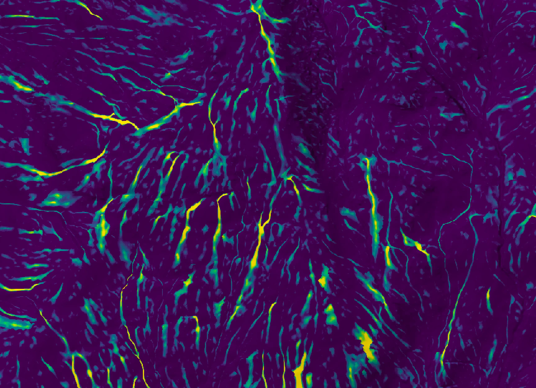
The UDSA (see image below) is defined for a grid cell as the number of upslope cells with a WI value higher than the current cell. Areas with non-zero UDSA are likely to have saturation deficits that are at least partly satisfied by local re-infiltation of overland flow from upslope areas. These non-zero UDSA cells are key sites causing the hydrologic disconnectivity of the catchment during certain conditions.
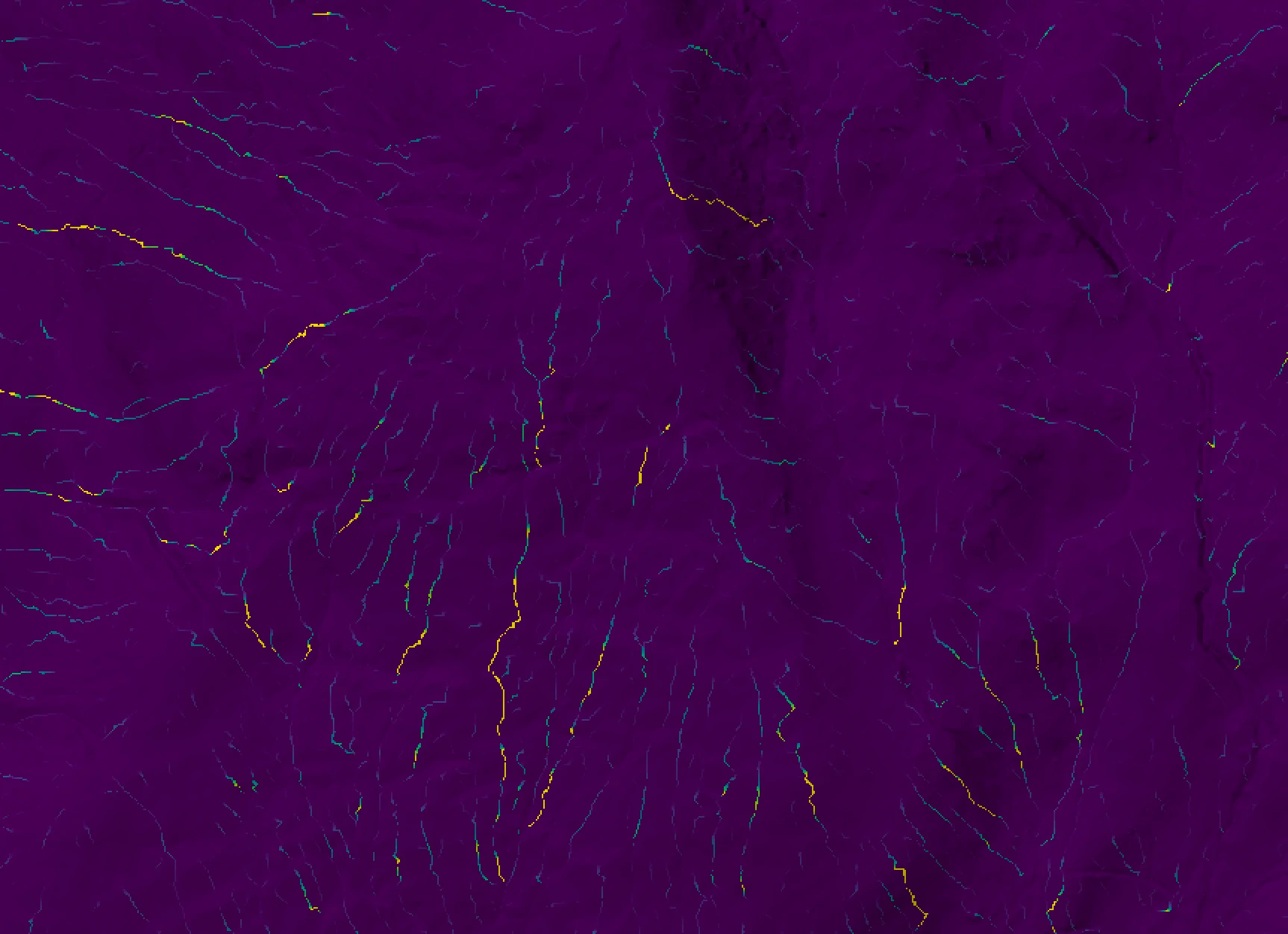
In the original Lane et al. (2004) NI paper, the authors state that the calculation of the index requires a unique, single downslope flow path for each grid cell. Therefore, the authors used the D8 single-direction flow algorithm to calculate NI. While the D8 method works well to model flow in convergent and channelized areas, it is generally recognized as a poor method for estimating WI on hillslopes, where divergent, non-chanellized flow dominates. Furthermore, the use of the D8 algorithm implied that the only way that WI can decrease downslope is for slope gradient to decrease, since specific contributing area only increases downslope with the D8 method. However, theoretically, WI may also decrease downslope due to flow dispersion, which allows for the upslope area (a surrogate for discharge) to be spread over a larger downslope dispersal area. The original NI formulation could not account for this effect.
Thus, in the implementation of the HydrologicConnectivity tool, WI is first calculated using the multiple flow-direction (MFD) algorithm described by Quinn et al. (1995), which is commonly used to estimate WI. While this implies that there are a multitude of potential flow pathways connecting each grid cell to a downstream location, in reality, if the flow path that follows the path of maximum WI issuing from a cell experiences a reduction in WI (to the point where it becomes less than the issuing cell's WI), then we can safely assume that re-infiltration occurs and the issuing cell is at times disconnected from downslope sites. Thus, after WI has been estimated using the QuinnFlowAccumulation algorithm, flow directions, which are used to calculate upslope and downslope flow paths for calculating the two indices, are approximated by identifying the downslope neighbour of highest WI value for each grid cell.
Operation
The user must specify the name of the input digital elevation model (DEM; --dem), and the output DUL and
UDSA rasters (--output1 and --output2). The DEM must have been hydrologically
corrected to remove all spurious depressions and flat areas. DEM pre-processing is usually achived using
either the BreachDepressions (also BreachDepressionsLeastCost) or FillDepressions tool. The
remaining two parameters are associated with the calculation of the Quinn et al. (1995) flow accumulation (QuinnFlowAccumulation), used
to estimate WI. A value must be specified for the exponent parameter
(--exponent), a number that controls the degree of dispersion in the flow-accumulation grid. A lower
value yields greater apparent flow dispersion across divergent hillslopes. The exponent value (h) should probably be
less than 10.0 and values between 1 and 2 are most common. The following equations are used to calculate the
portion flow (Fi) given to each neighbour, i:
Fi = Li(tanβ)p / Σi=1n[Li(tanβ)p]
p = (A / threshold + 1)h
Where Li is the contour length, and is 0.5×grid size for cardinal directions and 0.354×grid size for
diagonal directions, n = 8, and represents each of the eight neighbouring grid cells, and, A is the flow accumultation value assigned to the current grid cell, that is being
apportioned downslope. The non-dispersive, channel initiation threshold (--threshold) is a flow-accumulation
value (measured in upslope grid cells, which is directly proportional to area) above which flow dispersion is
no longer permited. Grid cells with flow-accumulation values above this threshold will have their flow routed
in a manner that is similar to the D8 single-flow-direction algorithm, directing all flow towards the steepest
downslope neighbour. This is usually done under the assumption that flow dispersion, whilst appropriate on
hillslope areas, is not realistic once flow becomes channelized. Importantly, the --threshold parameter sets
the spatial extent of the stream network, with lower values resulting in more extensive networks.
References:
Beven K.J., Kirkby M.J., 1979. A physically-based, variable contributing area model of basin hydrology. Hydrological Sciences Bulletin 24: 43–69.
Lane, S.N., Brookes, C.J., Kirkby, M.J. and Holden, J., 2004. A network‐index‐based version of TOPMODEL for use with high‐resolution digital topographic data. Hydrological processes, 18(1), pp.191-201.
Quinn, P. F., K. J. Beven, Lamb, R. 1995. The in (a/tanβ) index: How to calculate it and how to use it within the topmodel framework. Hydrological processes 9(2): 161-182.
See Also: WetnessIndex, QuinnFlowAccumulation
Parameters:
| Flag | Description |
|---|---|
| -d, --dem | Name of the input DEM raster file; must be depressionless |
| --output1 | Name of the output downslope unsaturated length (DUL) file |
| --output2 | Name of the output upslope disconnected saturated area (UDSA) file |
| --exponent | Optional exponent parameter; default is 1.0 |
| --threshold | Optional convergence threshold parameter, in grid cells; default is infinity |
Python function:
wbt.hydrologic_connectivity(
    dem,
    output1,
    output2,
    exponent=1.0,
    threshold=None,
    callback=default_callback
)
Command-line Interface:
-./whitebox_tools -r=HydrologicConnectivity --dem=DEM.tif ^
--output1=DUL.tif --output2=UDSA.tif --exponent=1.1 ^
--threshold=10000
Source code is unavailable due to proprietary license.
Author: Whitebox Geospatial Inc. (c)
Created: 08/07/2021
Last Modified: 08/07/2021
ImpoundmentSizeIndex
This tool can be used to calculate the impoundment size index (ISI) from a digital elevation model (DEM).
The ISI is a land-surface parameter related to the size of the impoundment that would result from inserting
a dam of a user-specified maximum length (--damlength) into each DEM grid cell. The tool requires the user
to specify the name of one or more of the possible outputs, which include the mean flooded depth (--out_mean),
the maximum flooded depth (--out_max), the flooded volume (--out_volume), the flooded area (--out_area),
and the dam height (--out_dam_height).
Please note that this tool performs an extremely complex and computationally intensive flow-accumulation operation.
As such, it may take a substantial amount of processing time and may encounter issues (including memory issues) when
applied to very large DEMs. It is not necessary to pre-process the input DEM (--dem) to remove topographic depressions
and flat areas. The internal flow-accumulation operation will not be confounded by the presence of these features.
Reference:
Lindsay, JB (2015) Modelling the spatial pattern of potential impoundment size from DEMs. Online resource: Whitebox Blog
See Also: InsertDams, StochasticDepressionAnalysis
Parameters:
| Flag | Description |
|---|---|
| -i, --dem | Input raster DEM file |
| --out_mean | Output mean flooded depth file |
| --out_max | Output maximum flooded depth file |
| --out_volume | Output flooded volume file |
| --out_area | Output flooded area file |
| --out_dam_height | Output dam height file |
| --damlength | Maximum length of the dam |
Python function:
wbt.impoundment_size_index(
    dem,
    damlength,
    out_mean=None,
    out_max=None,
    out_volume=None,
    out_area=None,
    out_dam_height=None,
    callback=default_callback
)
Command-line Interface:
>>./whitebox_tools -r=ImpoundmentSizeIndex -v ^
--wd="/path/to/data/" --dem=DEM.tif -o=out.tif ^
--out_type='max depth' --damlength=11
Author: Dr. John Lindsay
Created: 28/05/2018
Last Modified: 12/10/2018
InsertDams
This tool can be used to insert dams at one or more user-specified points (--dam_pts), and of a maximum length
(--damlength), within an input digital elevation model (DEM) (--dem). This tool can be thought of as providing
the impoundment feature that is calculated internally during a run of the the impoundment size index (ISI) tool for
a set of points of interest. from a (DEM).
Reference:
Lindsay, JB (2015) Modelling the spatial pattern of potential impoundment size from DEMs. Online resource: Whitebox Blog
See Also: ImpoundmentSizeIndex, StochasticDepressionAnalysis
Parameters:
| Flag | Description |
|---|---|
| -i, --dem | Input raster DEM file |
| --dam_pts | Input vector dam points file |
| -o, --output | Output file |
| --damlength | Maximum length of the dam |
Python function:
wbt.insert_dams(
    dem,
    dam_pts,
    output,
    damlength,
    callback=default_callback
)
Command-line Interface:
>>./whitebox_tools -r=InsertDams -v --wd="/path/to/data/" ^
--dem=DEM.tif --dam_pts=dams.shp -o=out.tif --damlength=11
Author: Dr. John Lindsay
Created: 19/02/2020
Last Modified: 20/02/2020
Isobasins
This tool can be used to divide a landscape into a group of nearly equal-sized watersheds, known as isobasins.
The user must specify the name (--dem) of a digital elevation model (DEM), the output raster name (--output),
and the isobasin target area (--size) specified in units of grid cells. The DEM must have been hydrologically
corrected to remove all spurious depressions and flat areas. DEM pre-processing is usually achieved using either
the BreachDepressions or FillDepressions tool. Several temporary rasters are created during the execution
and stored in memory of this tool.
The tool can optionally (--connections) output a CSV table that contains the upstream/downstream connections
among isobasins. That is, this table will identify the downstream basin of each isobasin, or will list N/A in
the event that there is no downstream basin, i.e. if it drains to an edge. Additionally, the CSV file will contain
information about the number of grid cells in each isobasin and the isobasin outlet's row and column number and
flow direction. The output CSV file will have the same name as the output raster, but with a *.csv file extension.
See Also: Watershed, Basins, BreachDepressions, FillDepressions
Parameters:
| Flag | Description |
|---|---|
| -i, --dem | Input raster DEM file |
| -o, --output | Output raster file |
| --size | Target basin size, in grid cells |
| --connections | Output upstream-downstream flow connections among basins? |
Python function:
wbt.isobasins(
    dem,
    output,
    size,
    connections=False,
    callback=default_callback
)
Command-line Interface:
>>./whitebox_tools -r=Isobasins -v --wd="/path/to/data/" ^
--dem=DEM.tif -o=output.tif --size=1000
Author: Dr. John Lindsay
Created: 03/12/2017
Last Modified: 24/07/2020
JensonSnapPourPoints
The JensonSnapPourPoints tool can be used to move the location of vector pour points (i.e. outlets used in a Watershed
operation) (--pour_pts) to the location coincident with the nearest stream cell (--stream) value within
a specified maximum distance (--snap_dist). The pour points file (--pour_pts) must be a vector file of Point ShapeType.
If the output of the JensonSnapPourPoints tool is to be used with the Watershed tool, the streams raster should
be generated by extracting the streams using the D8FlowAccumulation algorithm. The snap distance (--snap_dist), measured
in map units (e.g meters), must also be specified. This distance will serve as the search radius placed around each pour
point during the search for the nearst stream cell.
Lindsay et al. (2008) provide a detailed discussion of the JensonSnapPourPoints technique, and other less sophisticated but commonly used techniques (SnapPourPoints) for adjusting pour point locations used in watershedding operations. In most cases, the JensonSnapPourPoints tool should be preferred over SnapPourPoints for applications of repositioning outlet points used in watershedding operations onto the digital stream lines contained in local drainage direction rasters. Jenson's method relocates outlet points to the nearest stream cell while SnapPourPoints relocated outlets to the largest stream (designated by the largest flow accumulation value). In the common situation where outlet cells are position near the confluence point of smaller tributary streams, the SnapPourPoints tool may re-position outlets on the main-trunk stream, which will result in watershed delineation of incorrect sub-basins.
Reference:
Jenson, S. K. (1991), Applications of hydrological information automati-cally extracted from digital elevation models, Hydrological Processes, 5, 31–44, doi:10.1002/hyp.3360050104.
Lindsay JB, Rothwell JJ, and Davies H. 2008. Mapping outlet points used for watershed delineation onto DEM-derived stream networks, Water Resources Research, 44, W08442, doi:10.1029/2007WR006507.
See Also: Watershed, SnapPourPoints, D8FlowAccumulation
Parameters:
| Flag | Description |
|---|---|
| --pour_pts | Input vector pour points (outlet) file |
| --streams | Input raster streams file |
| -o, --output | Output vector file |
| --snap_dist | Maximum snap distance in map units |
Python function:
wbt.jenson_snap_pour_points(
    pour_pts,
    streams,
    output,
    snap_dist,
    callback=default_callback
)
Command-line Interface:
>>./whitebox_tools -r=JensonSnapPourPoints -v ^
--wd="/path/to/data/" --pour_pts='pour_pts.shp' ^
--streams='streams.tif' -o='output.shp' --snap_dist=15.0
Author: Dr. John Lindsay
Created: 27/06/2017
Last Modified: 12/10/2018
LongestFlowpath
This tool delineates the longest flowpaths for a group of subbasins or watersheds.
Flowpaths are initiated along drainage divides and continue along the D8-defined
flow direction until either the subbasin outlet or DEM edge is encountered. Each input
subbasin/watershed will have an associated vector flowpath in the output image. LongestFlowpath
is similar to the r.lfp plugin tool for GRASS GIS. The length of the longest flowpath
draining to an outlet is related to the time of concentration, which is a parameter
used in certain hydrological models.
The user must input the filename of a digital elevation model (DEM), a basins raster, and the output vector. The DEM must be depressionless and should have been pre-processed using the BreachDepressions or FillDepressions tool. The basins raster must contain features that are delineated by categorical (integer valued) unique identifier values. All non-NoData, non-zero valued grid cells in the basins raster are interpreted as belonging to features. In practice, this tool is usual run using either a single watershed, a group of contiguous non-overlapping watersheds, or a series of nested subbasins. These are often derived using the Watershed tool, based on a series of input outlets, or the Subbasins tool, based on an input stream network. If subbasins are input to LongestFlowpath, each traced flowpath will include only the non-overlapping portions within nested areas. Therefore, this can be a convenient method of delineating the longest flowpath to each bifurcation in a stream network.
The output vector file will contain fields in the attribute table that identify the associated basin unique identifier (BASIN), the elevation of the flowpath source point on the divide (UP_ELEV), the elevation of the outlet point (DN_ELEV), the length of the flowpath (LENGTH), and finally, the average slope (AVG_SLOPE) along the flowpath, measured as a percent grade.
See Also: MaxUpslopeFlowpathLength, BreachDepressions, FillDepressions, Watershed, Subbasins
Parameters:
| Flag | Description |
|---|---|
| -i, --dem | Input raster DEM file |
| --basins | Input raster basins file |
| -o, --output | Output vector file |
Python function:
wbt.longest_flowpath(
    dem,
    basins,
    output,
    callback=default_callback
)
Command-line Interface:
>>./whitebox_tools -r=LongestFlowpath -v ^
--wd="/path/to/data/" -i=DEM.tif --basins=basins.tif ^
-o=output.tif
Author: Dr. John Lindsay
Created: 29/10/2018
Last Modified: 29/10/2018
LowPointsOnHeadwaterDivides
Note this tool is part of a WhiteboxTools extension product. Please visit Whitebox Geospatial Inc. for information about purchasing a license activation key (https://www.whiteboxgeo.com/extension-pricing/).
This tool locates low points, or passes, on the drainage divides between subbasins that are situated on headwater divides. A subbasin is the catchment draining to a link in a stream network. A headwater catchment is the portion of a subbasin that drains to the channel head. Only first-order streams contain channel heads and headwater catchments are sometimes referred to as zero-order basins. The lowest points along a zero-order catchment is likely to coincide with mountain passes in alpine environments.
The user must input a depressionless DEM (i.e. a DEM that has been pre-processed to remove all topographic depressions) and a raster stream network. The tool will work best if the raster stream network, generally derived by thresholding a flow-accumulation raster, is processed to remove shorter headwater streams. You can use the RemoveShortStreams tool remove shorter streams in the input raster. It is recommended to remove streams shorter than 2 or 3 grid cells in length. The algorithm proceeds by first deriving the D8 flow pointer from the input DEM. It then identifies all channel head cells in the input streams raster and the zero-order basins that drain to them. The stream network is then processed to assign a unique identifier to each segment, which is then used to extract subbasins. Lastly, zero-order basin edge cells are identified and the location of lowest grid cells for each pair of neighbouring basins is entered into the output vector file.
See Also: RemoveShortStreams
Parameters:
| Flag | Description |
|---|---|
| -d, --dem | Name of the input DEM raster file |
| --streams | Name of the input stream channel raster file |
| -o, --output | Name of the output vector file |
Python function:
wbt.low_points_on_headwater_divides(
    dem,
    streams,
    output,
    callback=default_callback
)
Command-line Interface:
-./whitebox_tools -r=LowPointsOnHeadwaterDivides -i=input.tif ^
-s=streams.tif -o=new.tif
Source code is unavailable due to proprietary license.
Author: Whitebox Geospatial Inc. (c)
Created: 12/04/2021
Last Modified: 12/04/2021
MaxUpslopeFlowpathLength
This tool calculates the maximum length of the flowpaths that run through each grid cell (in map horizontal
units) in an input digital elevation model (--dem). The tool works by first calculating the D8 flow pointer
(D8Pointer) from the input DEM. The DEM must be depressionless and should have been pre-processed using
the BreachDepressions or FillDepressions tool. The user must also specify the name of output raster (--output).
See Also: D8Pointer, BreachDepressions, FillDepressions, AverageUpslopeFlowpathLength, DownslopeFlowpathLength, DownslopeDistanceToStream
Parameters:
| Flag | Description |
|---|---|
| -i, --dem | Input raster DEM file |
| -o, --output | Output raster file |
Python function:
wbt.max_upslope_flowpath_length(
    dem,
    output,
    callback=default_callback
)
Command-line Interface:
>>./whitebox_tools -r=MaxUpslopeFlowpathLength -v ^
--wd="/path/to/data/" -i=DEM.tif -o=output.tif
Author: Dr. John Lindsay
Created: 25/06/2017
Last Modified: 28/10/2019
MaxUpslopeValue
This tool is used to can be used calculate the maximum upslope value, based on the values within an
input values raster (--values), along flow-paths, as calculated using the D8 flow method. The user must
specify the names of the input digital elevation model (DEM) file (--dem), from which the D8 flow
direction data will be calculated internally, and the output file (--output).
See Also: D8FlowAccumulation, D8Pointer
Parameters:
| Flag | Description |
|---|---|
| -d, --dem | Input DEM; it must be depressionless |
| --values | Name of the input values raster file |
| --output | Name of the output raster file |
Python function:
wbt.max_upslope_value(
    dem,
    values,
    output,
    callback=default_callback
)
Command-line Interface:
-./whitebox_tools -r=MaxUpslopeValue --dem=DEM.tif ^
--values=values.tif --output=out.tif
Author: Dr. John Lindsay
Created: 26/02/2022
Last Modified: 26/02/2022
MdInfFlowAccumulation
This tool is used to generate a flow accumulation grid (i.e. contributing area) using the MD-infinity algorithm
(Seibert and McGlynn, 2007). This algorithm is an examples of a multiple-flow-direction (MFD) method because the flow entering
each grid cell is routed to one or two downslope neighbour, i.e. flow divergence is permitted. The user must
specify the name of the input digital elevation model (--dem). The DEM should have been hydrologically corrected
to remove all spurious depressions and flat areas. DEM pre-processing is usually achieved using the
BreachDepressions or FillDepressions tool.
In addition to the input flow-pointer grid name, the user must specify the output type (--out_type). The output
flow-accumulation
can be 1) specific catchment area (SCA), which is the upslope contributing area divided by the contour length (taken
as the grid resolution), 2) total catchment area in square-metres, or 3) the number of upslope grid cells. The user
must also specify whether the output flow-accumulation grid should be log-tranformed, i.e. the output, if this option
is selected, will be the natural-logarithm of the accumulated area. This is a transformation that is often performed
to better visualize the contributing area distribution. Because contributing areas tend to be very high along valley
bottoms and relatively low on hillslopes, when a flow-accumulation image is displayed, the distribution of values on
hillslopes tends to be 'washed out' because the palette is stretched out to represent the highest values.
Log-transformation (--log) provides a means of compensating for this phenomenon. Importantly, however, log-transformed
flow-accumulation grids must not be used to estimate other secondary terrain indices, such as the wetness index, or
relative stream power index.
Grid cells possessing the NoData value in the input DEM raster are assigned the NoData value in the output flow-accumulation image. The output raster is of the float data type and continuous data scale.
Reference:
Seibert, J. and McGlynn, B.L., 2007. A new triangular multiple flow direction algorithm for computing upslope areas from gridded digital elevation models. Water resources research, 43(4).
See Also: D8FlowAccumulation, FD8FlowAccumulation, QuinnFlowAccumulation, QinFlowAccumulation, DInfFlowAccumulation, MDInfFlowAccumulation, Rho8Pointer, BreachDepressionsLeastCost
Parameters:
| Flag | Description |
|---|---|
| -i, --dem | Input raster DEM file |
| -o, --output | Output raster file |
| --out_type | Output type; one of 'cells', 'specific contributing area' (default), and 'catchment area' |
| --exponent | Optional exponent parameter; default is 1.1 |
| --threshold | Optional convergence threshold parameter, in grid cells; default is infinity |
| --log | Optional flag to request the output be log-transformed |
| --clip | Optional flag to request clipping the display max by 1% |
Python function:
wbt.md_inf_flow_accumulation(
    dem,
    output,
    out_type="specific contributing area",
    exponent=1.1,
    threshold=None,
    log=False,
    clip=False,
    callback=default_callback
)
Command-line Interface:
>>./whitebox_tools -r=MDInfFlowAccumulation -v ^
--wd="/path/to/data/" --dem=DEM.tif -o=output.tif ^
--out_type='cells'
>>./whitebox_tools -r=MDInfFlowAccumulation ^
-v --wd="/path/to/data/" --dem=DEM.tif -o=output.tif ^
--out_type='catchment area' --exponent=1.5 --threshold=10000 ^
--log --clip
Author: Dr. John Lindsay
Created: 12/02/2020
Last Modified: 12/02/2020
NumInflowingNeighbours
This tool calculates the number of inflowing neighbours for each grid cell in a raster file. The user
must specify the names of an input digital elevation model (DEM) file (--dem) and the output raster
file (--output). The tool calculates the D8 pointer file internally in order to identify inflowing
neighbouring cells.
Grid cells in the input DEM that contain the NoData value will be assigned the NoData value in the output image. The output image is of the integer data type and continuous data scale.
See Also: NumDownslopeNeighbours, NumUpslopeNeighbours
Parameters:
| Flag | Description |
|---|---|
| -i, --dem | Input raster DEM file |
| -o, --output | Output raster file |
Python function:
wbt.num_inflowing_neighbours(
    dem,
    output,
    callback=default_callback
)
Command-line Interface:
>>./whitebox_tools -r=NumInflowingNeighbours -v ^
--wd="/path/to/data/" -i=DEM.tif -o=output.tif
Author: Dr. John Lindsay
Created: 25/06/2017
Last Modified: 12/10/2018
QinFlowAccumulation
This tool is used to generate a flow accumulation grid (i.e. contributing area) using the Qin et al. (2007) flow algorithm, not to be confused with the similarly named QuinnFlowAccumulation tool. This algorithm is an examples of a multiple-flow-direction (MFD) method because the flow entering each grid cell is routed to more than one downslope neighbour, i.e. flow divergence is permitted. It is based on a modification of the Freeman (1991; FD8FlowAccumulation) and Quinn et al. (1995; QuinnFlowAccumulation) methods. The Qin method relates the degree of flow dispersion from a grid cell to the local maximum downslope gradient. Specifically, steeper terrain experiences more convergent flow while flatter slopes experience more flow divergence.
The following equations are used to calculate the portion flow (Fi) given to each neighbour, i:
Fi = Li(tanβ)f(e) / Σi=1n[Li(tanβ)f(e)]
f(e) = min(e, eU) / eU × (pU - 1.1) + 1.1
Where Li is the contour length, and is 0.5×cell size for cardinal directions and 0.354×cell size for
diagonal directions, n = 8, and represents each of the eight neighbouring grid cells. The exponent f(e) controls
the proportion of flow allocated to each downslope neighbour of a grid cell, based on the local maximum downslope
gradient (e), and the user-specified upper boundary of e (eU; --max_slope), and the upper
boundary of the exponent (pU; --exponent), f(e). Note that the original Qin (2007)
implementation allowed for user-specified lower boundaries on the slope (eL) and exponent (pL)
parameters as well. In this implementation, these parameters are assumed to be 0.0 and 1.1 respectively, and are
not user adjustable. Also note, the --exponent parameter should be less than 50.0, as higher values may cause
numerical instability.
The user must specify the name (--dem) of the input digital elevation model (DEM) and the output file (--output).
The DEM must have been hydrologically corrected to remove all spurious depressions and flat areas. DEM
pre-processing is usually achieved using either the BreachDepressions (also BreachDepressionsLeastCost) or
FillDepressions tool.
The user-specified non-dispersive, channel initiation threshold (--threshold) is a flow-accumulation
value (measured in upslope grid cells, which is directly proportional to area) above which flow dispersion is
no longer permitted. Grid cells with flow-accumulation values above this area threshold will have their flow
routed in a manner that is similar to the D8 single-flow-direction algorithm, directing all flow towards the
steepest downslope neighbour. This is usually done under the assumption that flow dispersion, whilst appropriate
on hillslope areas, is not realistic once flow becomes channelized. Importantly, the --threshold parameter sets
the spatial extent of the stream network, with lower values resulting in more extensive networks.
In addition to the input DEM, output file (--output), and exponent, the user must also specify the output type (--out_type). The output flow-accumulation
can be: 1) cells (i.e. the number of inflowing grid cells), catchment area (i.e. the upslope area),
or specific contributing area (i.e. the catchment area divided by the flow width). The default value
is specific contributing area. The user must also specify whether the output flow-accumulation grid should be
log-tranformed (--log), i.e. the output, if this option is selected, will be the natural-logarithm of the
accumulated flow value. This is a transformation that is often performed to better visualize the
contributing area distribution. Because contributing areas tend to be very high along valley bottoms
and relatively low on hillslopes, when a flow-accumulation image is displayed, the distribution of
values on hillslopes tends to be 'washed out' because the palette is stretched out to represent the
highest values. Log-transformation provides a means of compensating for this phenomenon. Importantly,
however, log-transformed flow-accumulation grids must not be used to estimate other secondary terrain
indices, such as the wetness index (WetnessIndex), or relative stream power index (StreamPowerIndex).
Reference:
Freeman, T. G. (1991). Calculating catchment area with divergent flow based on a regular grid. Computers and Geosciences, 17(3), 413-422.
Qin, C., Zhu, A. X., Pei, T., Li, B., Zhou, C., & Yang, L. 2007. An adaptive approach to selecting a flow‐partition exponent for a multiple‐flow‐direction algorithm. International Journal of Geographical Information Science, 21(4), 443-458.
Quinn, P. F., K. J. Beven, Lamb, R. 1995. The in (a/tanβ) index: How to calculate it and how to use it within the topmodel framework. Hydrological Processes 9(2): 161-182.
See Also: D8FlowAccumulation, QuinnFlowAccumulation, FD8FlowAccumulation, DInfFlowAccumulation, MDInfFlowAccumulation, Rho8Pointer, WetnessIndex
Parameters:
| Flag | Description |
|---|---|
| -d, --dem | Name of the input DEM raster file; must be depressionless |
| --output | Name of the output raster file |
| --out_type | Output type; one of 'cells', 'specific contributing area' (default), and 'catchment area' |
| --exponent | Optional upper-bound exponent parameter; default is 10.0 |
| --max_slope | Optional upper-bound slope parameter, in degrees (0-90); default is 45.0 |
| --threshold | Optional convergence threshold parameter, in grid cells; default is infinity |
| --log | Log-transform the output values? |
| --clip | Optional flag to request clipping the display max by 1% |
Python function:
wbt.qin_flow_accumulation(
    dem,
    output,
    out_type="specific contributing area",
    exponent=10.0,
    max_slope=45.0,
    threshold=None,
    log=False,
    clip=False,
    callback=default_callback
)
Command-line Interface:
-./whitebox_tools -r=QinFlowAccumulation --dem=DEM.tif ^
--output=QinMFD.tif --out_type='specific contributing area' ^
--exponent=15.0 --max_slope=30.0 --threshold=10000
Author: Dr. John Lindsay
Created: 15/07/2021
Last Modified: 15/07/2021
QuinnFlowAccumulation
This tool is used to generate a flow accumulation grid (i.e. contributing area) using the Quinn et al. (1995)
flow algorithm, sometimes called QMFD or QMFD2, and not to be confused with the similarly named QinFlowAccumulation tool. This algorithm is an examples of a multiple-flow-direction (MFD) method because the flow entering each
grid cell is routed to more than one downslope neighbour, i.e. flow divergence is permitted. The user must specify the
name (--dem) of the input digital elevation model (DEM). The DEM must have been hydrologically
corrected to remove all spurious depressions and flat areas. DEM pre-processing is usually achieved using
either the BreachDepressions (also BreachDepressionsLeastCost) or FillDepressions tool. A value must also be specified for the exponent parameter
(--exponent), a number that controls the degree of dispersion in the resulting flow-accumulation grid. A lower
value yields greater apparent flow dispersion across divergent hillslopes. The exponent value (h) should probably be
less than 50.0, as higher values may cause numerical instability, and values between 1 and 2 are most common.
The following equations are used to calculate the portion flow (Fi) given to each neighbour, i:
Fi = Li(tanβ)p / Σi=1n[Li(tanβ)p]
p = (A / threshold + 1)h
Where Li is the contour length, and is 0.5×cell size for cardinal directions and 0.354×cell size for
diagonal directions, n = 8, and represents each of the eight neighbouring grid cells, and, A is the flow accumulation value assigned to the current grid cell, that is being
apportioned downslope. The non-dispersive, channel initiation threshold (--threshold) is a flow-accumulation
value (measured in upslope grid cells, which is directly proportional to area) above which flow dispersion is
no longer permitted. Grid cells with flow-accumulation values above this threshold will have their flow routed
in a manner that is similar to the D8 single-flow-direction algorithm, directing all flow towards the steepest
downslope neighbour. This is usually done under the assumption that flow dispersion, whilst appropriate on
hillslope areas, is not realistic once flow becomes channelized. Importantly, the --threshold parameter sets
the spatial extent of the stream network, with lower values resulting in more extensive networks.
In addition to the input DEM, output file (--output), and exponent, the user must also specify the output type (--out_type). The output flow-accumulation
can be: 1) cells (i.e. the number of inflowing grid cells), catchment area (i.e. the upslope area),
or specific contributing area (i.e. the catchment area divided by the flow width). The default value
is specific contributing area. The user must also specify whether the output flow-accumulation grid should be
log-transformed (--log), i.e. the output, if this option is selected, will be the natural-logarithm of the
accumulated flow value. This is a transformation that is often performed to better visualize the
contributing area distribution. Because contributing areas tend to be very high along valley bottoms
and relatively low on hillslopes, when a flow-accumulation image is displayed, the distribution of
values on hillslopes tends to be 'washed out' because the palette is stretched out to represent the
highest values. Log-transformation provides a means of compensating for this phenomenon. Importantly,
however, log-transformed flow-accumulation grids must not be used to estimate other secondary terrain
indices, such as the wetness index (WetnessIndex), or relative stream power index (StreamPowerIndex). The
Quinn et al. (1995) algorithm is commonly used to calculate wetness index.
Reference:
Quinn, P. F., K. J. Beven, Lamb, R. 1995. The in (a/tanβ) index: How to calculate it and how to use it within the topmodel framework. Hydrological Processes 9(2): 161-182.
See Also: D8FlowAccumulation, QinFlowAccumulation, FD8FlowAccumulation, DInfFlowAccumulation, MDInfFlowAccumulation, Rho8Pointer, WetnessIndex
Parameters:
| Flag | Description |
|---|---|
| -d, --dem | Name of the input DEM raster file; must be depressionless |
| --output | Name of the output raster file |
| --out_type | Output type; one of 'cells', 'specific contributing area' (default), and 'catchment area' |
| --exponent | Optional exponent parameter; default is 1.0 |
| --threshold | Optional convergence threshold parameter, in grid cells; default is infinity |
| --log | Log-transform the output values? |
| --clip | Optional flag to request clipping the display max by 1% |
Python function:
wbt.quinn_flow_accumulation(
    dem,
    output,
    out_type="specific contributing area",
    exponent=1.0,
    threshold=None,
    log=False,
    clip=False,
    callback=default_callback
)
Command-line Interface:
-./whitebox_tools -r=QuinnFlowAccumulation --dem=DEM.tif ^
--output=QMFD.tif --out_type='specific contributing area' ^
--exponent=1.1 --threshold=10000
Author: Dr. John Lindsay
Created: 09/07/2021
Last Modified: 15/07/2021
RaiseWalls
This tool is used to increment the elevations in a digital elevation model (DEM) along
the boundaries of a vector lines or polygon layer. The user must specify the name of the
raster DEM (--dem), the vector file (--input), the output file name (--output), the
increment height (--height), and an optional breach lines vector layer (--breach).
The breach lines layer can be used to breach a whole in the raised walls at intersections
with the wall layer.
Parameters:
| Flag | Description |
|---|---|
| -i, walls, --input | Input vector lines or polygons file |
| --breach | Optional input vector breach lines |
| --dem | Input raster DEM file |
| -o, --output | Output raster file |
| --height | Wall height |
Python function:
wbt.raise_walls(
    i,
    dem,
    output,
    breach=None,
    height=100.0,
    callback=default_callback
)
Command-line Interface:
>>./whitebox_tools -r=RaiseWalls -v --wd="/path/to/data/" ^
-i=watershed.shp --dem=dem.tif -o=output.tif ^
--height=25.0
>>./whitebox_tools -r=RaiseWalls -v ^
--wd="/path/to/data/" -i=watershed.shp --breach=outlet.shp ^
--dem=dem.tif -o=output.tif --height=25.0
Author: Dr. John Lindsay
Created: 22/04/2018
Last Modified: 22/10/2019
Rho8FlowAccumulation
This tool is used to generate a flow accumulation grid (i.e. contributing area) using the Fairfield and Leymarie (1991)
flow algorithm, often called Rho8. Like the D8 flow method, this algorithm is an examples of a single-flow-direction (SFD) method because the flow entering each
grid cell is routed to only one downslope neighbour, i.e. flow divergence is not permitted. The user must specify the
name of the input file (--input), which may be either a digital elevation model (DEM) or a Rho8 pointer file (see Rho8Pointer). If a DEM is input, it must have been hydrologically
corrected to remove all spurious depressions and flat areas. DEM pre-processing is usually achieved using
either the BreachDepressions (also BreachDepressionsLeastCost) or FillDepressions tool.
In addition to the input and output (--output)files, the user must also specify the output type (--out_type). The output flow-accumulation
can be: 1) cells (i.e. the number of inflowing grid cells), catchment area (i.e. the upslope area),
or specific contributing area (i.e. the catchment area divided by the flow width). The default value
is specific contributing area. The user must also specify whether the output flow-accumulation grid should be
log-tranformed (--log), i.e. the output, if this option is selected, will be the natural-logarithm of the
accumulated flow value. This is a transformation that is often performed to better visualize the
contributing area distribution. Because contributing areas tend to be very high along valley bottoms
and relatively low on hillslopes, when a flow-accumulation image is displayed, the distribution of
values on hillslopes tends to be 'washed out' because the palette is stretched out to represent the
highest values. Log-transformation provides a means of compensating for this phenomenon. Importantly,
however, log-transformed flow-accumulation grids must not be used to estimate other secondary terrain
indices, such as the wetness index (WetnessIndex), or relative stream power index (StreamPowerIndex).
If a Rho8 pointer is used as the input raster, the user must specify this (--pntr). Similarly,
if a pointer input is used and the pointer follows the Esri pointer convention, rather than the
default WhiteboxTools convension for pointer files, then this must also be specified (--esri_pntr).
Reference:
Fairfield, J., and Leymarie, P. 1991. Drainage networks from grid digital elevation models. Water Resources Research, 27(5), 709-717.
See Also: Rho8Pointer, D8FlowAccumulation, QinFlowAccumulation, FD8FlowAccumulation, DInfFlowAccumulation, MDInfFlowAccumulation, WetnessIndex
Parameters:
| Flag | Description |
|---|---|
| -i, --input | Input DEM or Rho8 pointer file; if a DEM is used, it must be depressionless |
| --output | Name of the output raster file |
| --out_type | Output type; one of 'cells', 'specific contributing area' (default), and 'catchment area' |
| --log | Log-transform the output values? |
| --clip | Optional flag to request clipping the display max by 1% |
| --pntr | Is the input raster a Rho8 flow pointer rather than a DEM? |
| --esri_pntr | Does the input Rho8 pointer use the ESRI style scheme? |
Python function:
wbt.rho8_flow_accumulation(
    i,
    output,
    out_type="specific contributing area",
    log=False,
    clip=False,
    pntr=False,
    esri_pntr=False,
    callback=default_callback
)
Command-line Interface:
-./whitebox_tools -r=Rho8FlowAccumulation --dem=DEM.tif ^
--output=Rho8.tif --out_type='specific contributing area'
Author: Dr. John Lindsay
Created: 25/08/2021
Last Modified: 29/08/2021
Rho8Pointer
This tool is used to generate a flow pointer grid (i.e. flow direction) using the stochastic
Rho8 (J. Fairfield and P. Leymarie, 1991) algorithm. Like the D8 flow algorithm (D8Pointer),
Rho8 is a single-flow-direction (SFD) method because the flow entering each grid cell is routed
to only one downslope neighbour, i.e. flow divergence is not permitted. The user must specify the
name of a digital elevation model (DEM) file (--dem) that has been hydrologically corrected to
remove all spurious depressions and flat areas (BreachDepressions, FillDepressions). The
output of this tool (--output) is often used as the input to the Rho8FlowAccumulation tool.
By default, the Rho8 flow pointers use the following clockwise, base-2 numeric index convention:
| . | . | . |
|---|---|---|
| 64 | 128 | 1 |
| 32 | 0 | 2 |
| 16 | 8 | 4 |
Notice that grid cells that have no lower neighbours are assigned a flow direction of zero. In a DEM that has been
pre-processed to remove all depressions and flat areas, this condition will only occur along the edges of the grid.
If the pointer file contains ESRI flow direction values instead, the --esri_pntr parameter must be specified.
Grid cells possessing the NoData value in the input DEM are assigned the NoData value in the output image.
Memory Usage
The peak memory usage of this tool is approximately 10 bytes per grid cell.
References:
Fairfield, J., and Leymarie, P. 1991. Drainage networks from grid digital elevation models. Water Resources Research, 27(5), 709-717.
See Also: Rho8FlowAccumulation, D8Pointer, FD8Pointer, DInfPointer, BreachDepressions, FillDepressions
Parameters:
| Flag | Description |
|---|---|
| -i, --dem | Input raster DEM file |
| -o, --output | Output raster file |
| --esri_pntr | D8 pointer uses the ESRI style scheme |
Python function:
wbt.rho8_pointer(
    dem,
    output,
    esri_pntr=False,
    callback=default_callback
)
Command-line Interface:
>>./whitebox_tools -r=Rho8Pointer -v --wd="/path/to/data/" ^
--dem=DEM.tif -o=output.tif
Author: Dr. John Lindsay
Created: 16/07/2017
Last Modified: 18/10/2019
RiverCenterlines
Note this tool is part of a WhiteboxTools extension product. Please visit Whitebox Geospatial Inc. for information about purchasing a license activation key (https://www.whiteboxgeo.com/extension-pricing/).
This tool can map river centerlines, or medial-lines, from input river rasters (--input). The input river (or
water) raster is often derived from an image classification performed on multispectral satellite imagery. The
river raster must be a Boolean (1 for water, 0/NoData for not-water) and can be derived either by reclassifying
the classification output, or derived using a 1-class classification procedure. For example, using the
ParallelepipedClassification tool, it is possible to train the classifier using water training polygons,
and all other land classes will simply be left unclassified. It may be necessary to perform some pre-processing
on the water Boolean raster before input to the centerlines tool. For example, you may need to remove smaller
water polygons associated with small lakes and ponds, and you may want to remove small islands from the remaining
water features. This tool will often create a bifurcating vector path around islands within rivers, even if those
islands are a single-cell in size. The RemoveRasterPolygonHoles tool can be used to remove islands in the
water raster that are smaller than a user-specified size. The user must also specify the minimum line length
(--min_length), which determines the level of detail in the final rivers map. For example, in the first iamge
below, a value of 30 grid cells was used for the --min_length parameter, while a value of 5 was used in the
second image, which possesses far more (arguably too much) detail.
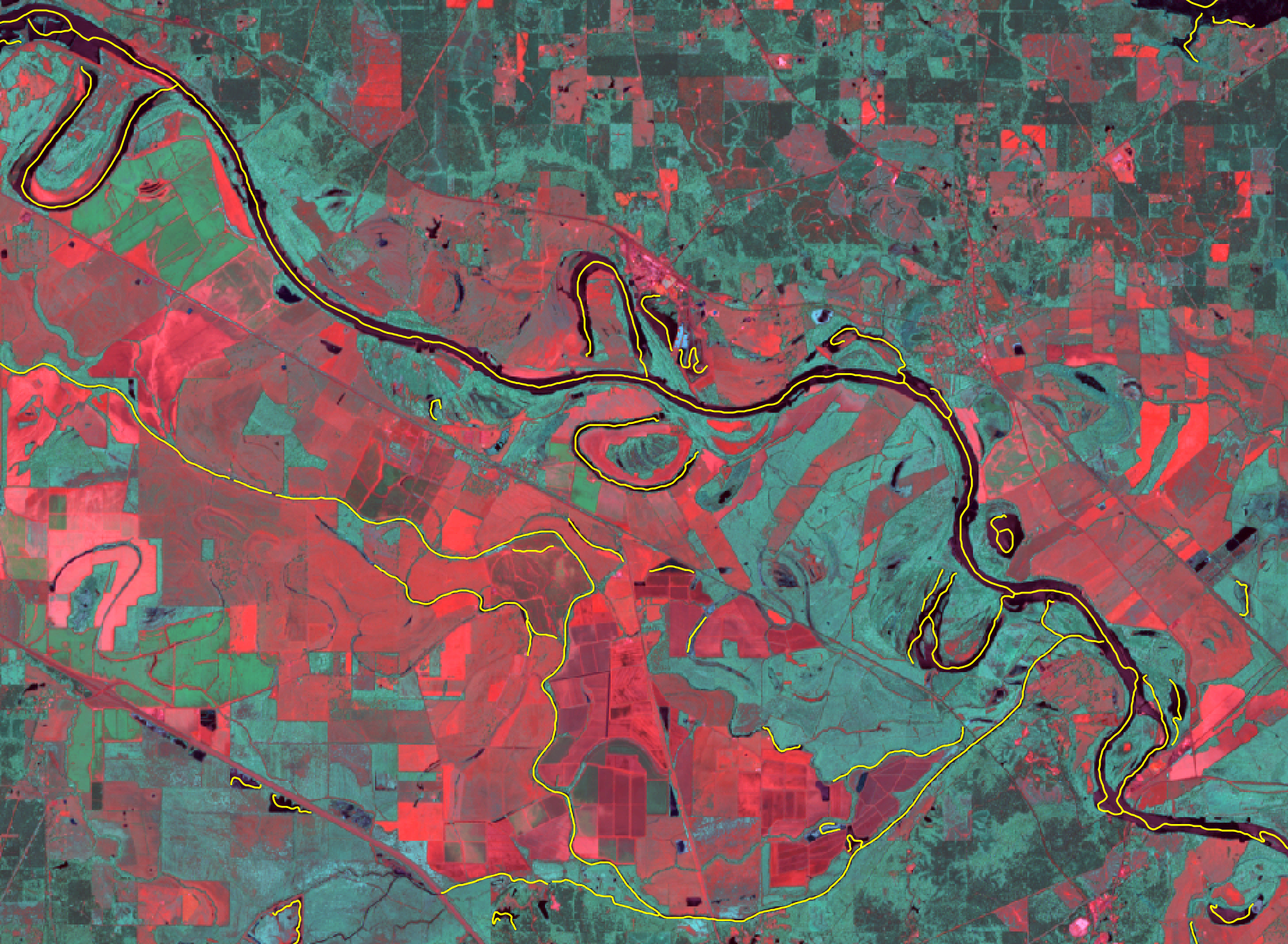
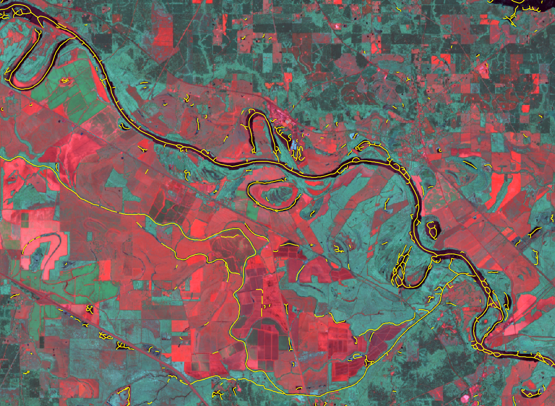
Lastly, the user must specify the --radius parameter value. At times, the tool will be able to connect distant
water polygons that are part of the same feature and this parameter determines the size of the search radius
used to identify separated line end-nodes that are candidates for connection. It is advisable that this value
not be set too high, or else unexpected connections may be made between unrelated water features. However, a value
of between 1 and 5 can produce satisfactory results. Experimentation may be needed to find an appropriate value
for any one data set however. The image below provides an example of this characteristic of the tool, where
the resulting vector stream centerline passes through disconnected raster water polygons in the underlying input
image in four locations.
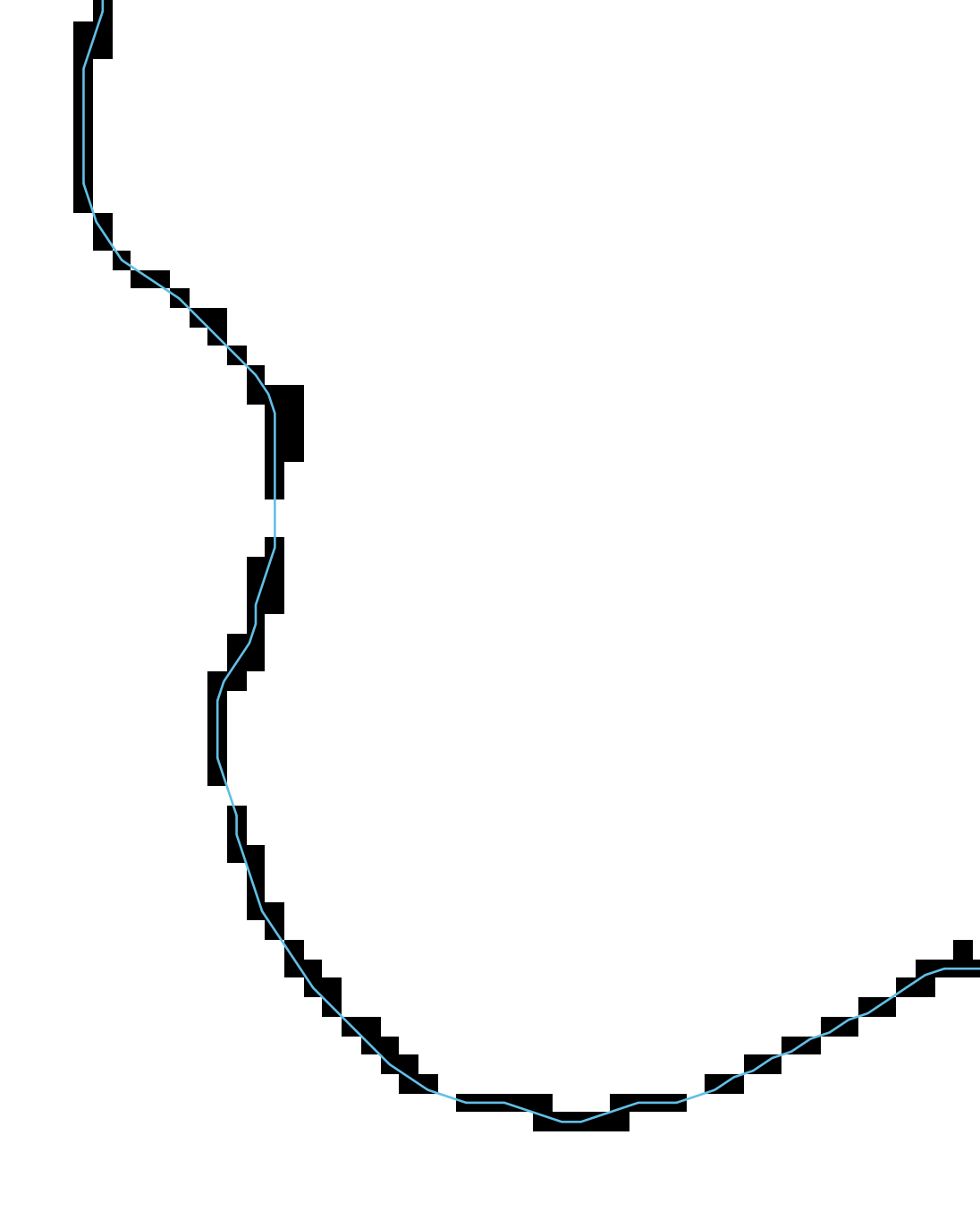
Here is a video that demonstrates how to apply this tool to map river center-lines taken from a water raster created by classifying a Sentinel-2 multi-spectral satellite imagery data set.
See Also: ParallelepipedClassification, RemoveRasterPolygonHoles
Parameters:
| Flag | Description |
|---|---|
| -i, --input | Name of the input raster image file |
| -o, --output | Name of the output vector lines file |
| --min_length | Minimum line length, in grid cells |
| --radius | Search radius for joining distant endnodes, in grid cells |
Python function:
wbt.river_centerlines(
    i,
    output,
    min_length=3,
    radius=4,
    callback=default_callback
)
Command-line Interface:
>> ./whitebox_tools -r=RiverCenterlines -i=water.tif ^
-o=river_centerlines.shp --min_length=20 --radius=4
Source code is unavailable due to proprietary license.
Author: Whitebox Geospatial Inc. (c)
Created: 13/10/2022
Last Modified: 13/10/2022
Sink
This tool identifies each sink (i.e. topographic depression) in a raster digital elevation model (DEM). A sink, or depression, is a bowl-like landscape feature, which is characterized by interior drainage. Each identified sink in the input DEM is assigned a unique, non-zero, positive value in the output raster. The Sink tool essentially runs the FillDepressions tool followed by the Clump tool on all modified grid cells.
See Also: FillDepressions, Clump
Parameters:
| Flag | Description |
|---|---|
| -i, --dem, --input | Input raster DEM file |
| -o, --output | Output raster file |
| --zero_background | Flag indicating whether a background value of zero should be used |
Python function:
wbt.sink(
    i,
    output,
    zero_background=False,
    callback=default_callback
)
Command-line Interface:
>>./whitebox_tools -r=Sink -v --wd="/path/to/data/" ^
--dem=DEM.tif -o=filled_dem.tif --zero_background
Author: Dr. John Lindsay
Created: 01/07/2017
Last Modified: 05/12/2019
SnapPourPoints
The SnapPourPoints tool can be used to move the location of vector pour points (i.e. outlets used in a Watershed
operation) (--pour_pts) to the location coincident with the highest flow accumulation (--flow_accum) value within
a specified maximum distance (--snap_dist). The pour points file (--pour_pts) must be a vector file of Point ShapeType.
If the output of the SnapPourPoints tool is to be used with the Watershed tool, the flow accumulation raster should
be generated using the D8FlowAccumulation algorithm. The snap distance (--snap_dist), measured in map units (e.g.
meters), must also be specified. This distance will serve as the search radius placed around each pour point during the
search for the maximum flow accumulation. In general, each outlet will be relocated the distance specified by the snap
distance.
Lindsay et al. (2008) provide a detailed discussion of the SnapPourPoints technique, and other more sophisticated techniques for adjusting pour point locations used in watershedding operations including Jenson's snap pour points (JensonSnapPourPoints) method. In most cases, the JensonSnapPourPoints tool should be preferred for applications of repositioning outlet points used in watershedding operations onto the digital stream lines contained in local drainage direction rasters. Jenson's method relocates outlet points to the nearest stream cell while SnapPourPoints relocated outlets to the largest stream (designated by the largest flow accumulation value). In the common situation where outlet cells are position near the confluence point of smaller tributary streams, the SnapPourPoints tool may re-position outlets on the main-trunk stream, which will result in watershed delineation of incorrect sub-basins.
Reference:
Lindsay JB, Rothwell JJ, and Davies H. 2008. Mapping outlet points used for watershed delineation onto DEM-derived stream networks, Water Resources Research, 44, W08442, doi:10.1029/2007WR006507.
See Also: Watershed, JensonSnapPourPoints, D8FlowAccumulation
Parameters:
| Flag | Description |
|---|---|
| --pour_pts | Input vector pour points (outlet) file |
| --flow_accum | Input raster D8 flow accumulation file |
| -o, --output | Output vector file |
| --snap_dist | Maximum snap distance in map units |
Python function:
wbt.snap_pour_points(
    pour_pts,
    flow_accum,
    output,
    snap_dist,
    callback=default_callback
)
Command-line Interface:
>>./whitebox_tools -r=SnapPourPoints -v --wd="/path/to/data/" ^
--pour_pts='pour_pts.shp' --flow_accum='d8accum.tif' ^
-o='output.shp' --snap_dist=15.0
Author: Dr. John Lindsay
Created: 27/072017
Last Modified: 12/10/2018
StochasticDepressionAnalysis
This tool performs a stochastic analysis of depressions within a DEM, calculating the probability of each cell belonging to a depression. This land-surface parameter (pdep) has been widely applied in wetland and bottom-land mapping applications.
This tool differs from the original Whitebox GAT tool in a few significant ways:
-
The Whitebox GAT tool took an error histogram as an input. In practice people found it difficult to create this input. Usually they just generated a normal distribution in a spreadsheet using information about the DEM root-mean-square-error (RMSE). As such, this tool takes a RMSE input and generates the histogram internally. This is more convienent for most applications but loses the flexibility of specifying the error distribution more completely.
-
The Whitebox GAT tool generated the error fields using the turning bands method. This tool generates a random Gaussian error field with no spatial autocorrelation and then applies local spatial averaging using a Gaussian filter (the size of which depends of the error autocorrelation length input) to increase the level of autocorrelation. We use the Fast Almost Gaussian Filter of Peter Kovesi (2010), which uses five repeat passes of a mean filter, based on an integral image. This filter method is highly efficient. This results in a significant performance increase compared with the original tool.
-
Parts of the tool's workflow utilize parallel processing. However, the depression filling operation, which is the most time-consuming part of the workflow, is not parallelized.
In addition to the input DEM (--dem) and output pdep file name (--output), the user
must specify the nature of the error model, including the root-mean-square error (--rmse) and
the error field correlation length (--range, in map units). These parameters determine the statistical frequency
distribution and spatial characteristics of the modeled error fields added to the DEM in each
iteration of the simulation. The user must also specify the number of iterations (--iterations).
A larger number of iterations will produce a smoother pdep raster.
This tool creates several temporary rasters in memory and, as a result, is very memory hungry. This will necessarily limit the size of DEMs that can be processed on more memory-constrained systems. As a rough guide for usage, the computer system will need 6-10 times more memory than the file size of the DEM. If your computer possesses insufficient memory, you may consider splitting the input DEM apart into smaller tiles.
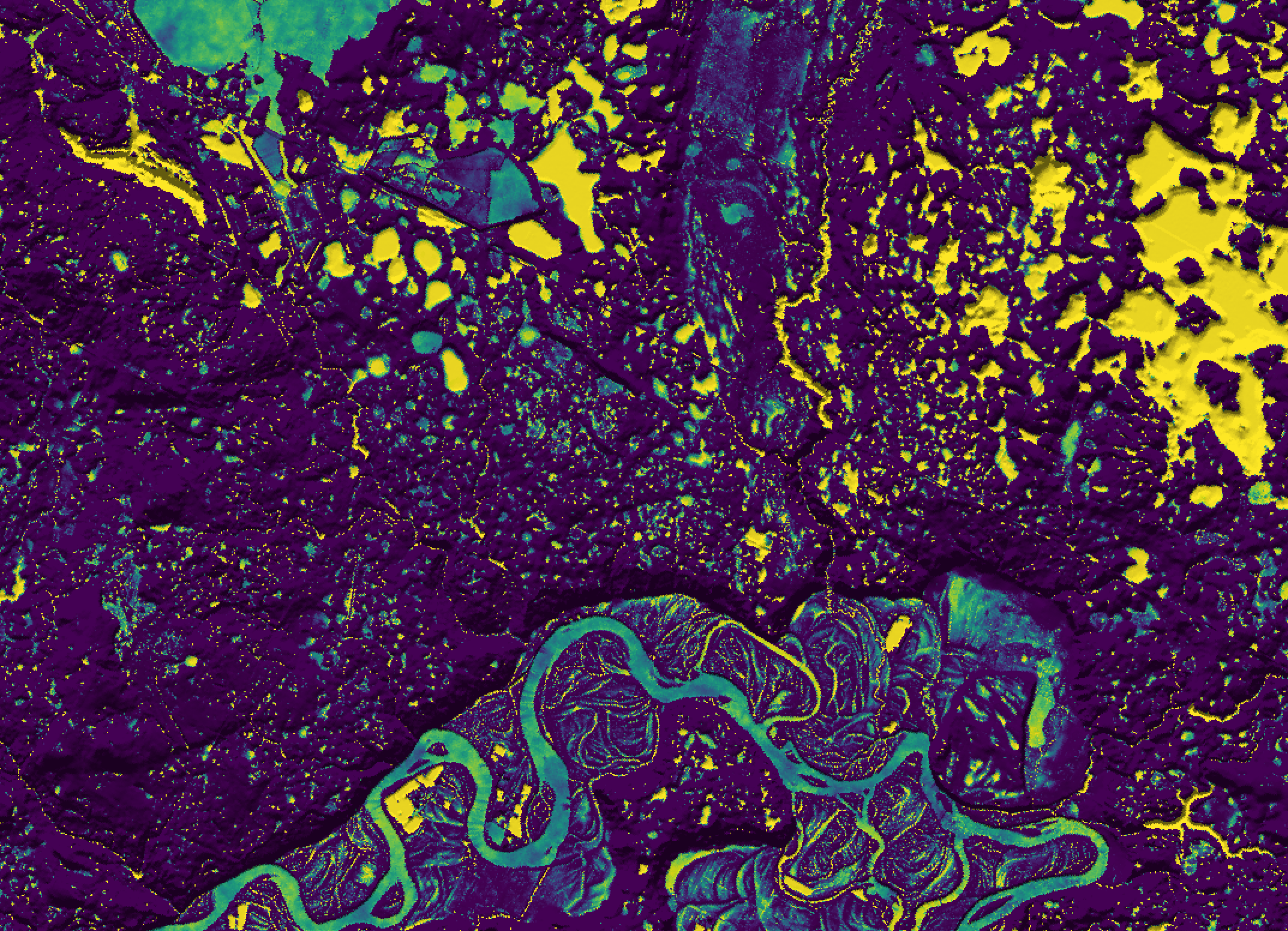
For a video demonstrating the application of the StochasticDepressionAnalysis tool, see this YouTube video.
Reference:
Lindsay, J. B., & Creed, I. F. (2005). Sensitivity of digital landscapes to artifact depressions in remotely-sensed DEMs. Photogrammetric Engineering & Remote Sensing, 71(9), 1029-1036.
See Also: ImpoundmentSizeIndex, FastAlmostGaussianFilter
Parameters:
| Flag | Description |
|---|---|
| -i, --dem | Input raster DEM file |
| -o, --output | Output file |
| --rmse | The DEM's root-mean-square-error (RMSE), in z units. This determines error magnitude |
| --range | The error field's correlation length, in xy-units |
| --iterations | The number of iterations |
Python function:
wbt.stochastic_depression_analysis(
    dem,
    output,
    rmse,
    range,
    iterations=100,
    callback=default_callback
)
Command-line Interface:
>>./whitebox_tools -r=StochasticDepressionAnalysis -v ^
--wd="/path/to/data/" --dem=DEM.tif -o=out.tif --rmse=10.0 ^
--range=850.0 --iterations=2500
Author: Dr. John Lindsay
Created: 11/05/2018
Last Modified: 29/03/2019
StrahlerOrderBasins
This tool will identify the catchment areas of each Horton-Strahler stream order link in a user-specified
stream network (--streams), i.e. the network's Strahler basins. The tool effectively performs a Horton-Strahler
stream ordering operation (HortonStreamOrder) followed by by a Watershed operation. The user must specify the name of a
flow pointer (flow direction) raster (--d8_pntr), a streams raster (--streams), and the output raster
(--output). The flow pointer and streams rasters should be generated using the D8Pointer algorithm. This
will require a depressionless DEM, processed using either the BreachDepressions or FillDepressions tool.
By default, the pointer raster is assumed to use the clockwise indexing method used by WhiteboxTools.
If the pointer file contains ESRI flow direction values instead, the --esri_pntr parameter must be specified.
NoData values in the input flow pointer raster are assigned NoData values in the output image.
See Also: HortonStreamOrder, Watershed, D8Pointer, BreachDepressions, FillDepressions
Parameters:
| Flag | Description |
|---|---|
| --d8_pntr | Input raster D8 pointer file |
| --streams | Input raster streams file |
| -o, --output | Output raster file |
| --esri_pntr | D8 pointer uses the ESRI style scheme |
Python function:
wbt.strahler_order_basins(
    d8_pntr,
    streams,
    output,
    esri_pntr=False,
    callback=default_callback
)
Command-line Interface:
>>./whitebox_tools -r=StrahlerOrderBasins -v ^
--wd="/path/to/data/" --d8_pntr='d8pntr.tif' ^
--streams='streams.tif' -o='output.tif'
Author: Dr. John Lindsay
Created: 13/07/2017
Last Modified: 18/10/2019
Subbasins
This tool will identify the catchment areas to each link in a user-specified stream network, i.e. the
network's sub-basins. Subbasins effectively performs a stream link ID operation (StreamLinkIdentifier) followed by
a Watershed operation. The user must specify the name of a flow pointer (flow direction) raster (--d8_pntr),
a streams raster (--streams), and the output raster (--output). The flow pointer and streams rasters should
be generated using the D8Pointer algorithm. This will require a depressionless DEM, processed using either
the BreachDepressions or FillDepressions tool.
Hillslopes are conceptually similar to sub-basins, except that sub-basins do not distinguish between the right-bank and left-bank catchment areas of stream links. The Sub-basins tool simply assigns a unique identifier to each stream link in a stream network.
By default, the pointer raster is assumed to use the clockwise indexing method used by WhiteboxTools.
If the pointer file contains ESRI flow direction values instead, the --esri_pntr parameter must be specified.
NoData values in the input flow pointer raster are assigned NoData values in the output image.
See Also: StreamLinkIdentifier, Watershed, Hillslopes, D8Pointer, BreachDepressions, FillDepressions
Parameters:
| Flag | Description |
|---|---|
| --d8_pntr | Input D8 pointer raster file |
| --streams | Input raster streams file |
| -o, --output | Output raster file |
| --esri_pntr | D8 pointer uses the ESRI style scheme |
Python function:
wbt.subbasins(
    d8_pntr,
    streams,
    output,
    esri_pntr=False,
    callback=default_callback
)
Command-line Interface:
>>./whitebox_tools -r=Subbasins -v --wd="/path/to/data/" ^
--d8_pntr='d8pntr.tif' --streams='streams.tif' ^
-o='output.tif'
Author: Dr. John Lindsay
Created: 01/07/2017
Last Modified: 13/02/2020
TopologicalBreachBurn
Note this tool is part of a WhiteboxTools extension product. Please visit Whitebox Geospatial Inc. for information about purchasing a license activation key (https://www.whiteboxgeo.com/extension-pricing/).
This tool performs a specialized form of stream burning, i.e. the practice of forcing the surface flow paths modelled from a digital elevation model (DEM) to match the pathway of a mapped vector stream network. Stream burning is a common flow enforcement technique used to correct surface drainage patterns derived from DEMs. The technique involves adjusting the elevations of grid cells that are coincident with the features of a vector hydrography layer, usually simply by lowering stream cell elevations by a constant offset value. This simple approach is used by the FillBurn tool, which suffers greatly from topological errors resulting from the mismatched scales of the hydrography and DEM data sets. These topological errors, which occur during the rasterization of the stream vector, result in inappropriate stream cell adjacencies (where two stream links appear to be beside one another in the stream raster with no space between) and collisions (where two stream links occupy the same cell in the stream raster). The TopologicalBreachBurn method uses total upstream channel length (TUCL) to prune the vector hydrography layer to a level of detail that matches the raster DEM grid resolution. Network pruning reduces the occurrence of erroneous stream piracy caused by the rasterization of multiple stream links to the same DEM grid cell. The algorithm also restricts flow, during the calculation of the D8 flow pointer raster output, within individual stream reaches, further reducing erroneous stream piracy. In situations where two vector stream features occupy the same grid cell, the new tool ensures that the larger stream, designated by higher TUCL, is given priority. TUCL-based priority minimizes the impact of the topological errors that occur during the stream rasterization process on modelled regional drainage patterns. Lindsay (2016) demonstrated that the TopologicalBreachBurn method produces highly accurate and scale-insensitive drainage patterns and watershed boundaries compared with FillBurn.
The tool requires two input layers, including the DEM (--dem) and mapped vector stream network (--streams). Note that
these two inputs must share the same map projection. The tool also produces four output rasters, including:
-
A rasterized version of the pruned stream network (
--out_streams). Network pruning is based on a TUCL threshold that is calculated as the optimal value that satisfies the combined objectives of maximizing the length of maintained streams and minimizing the number of collisions/adjacencies in the rasterized network. This optimization process is carried out using TUCL and stream length data calculated for each tributary in the network. A tributary connects a channel head and a downstream confluence/outlet in the stream network. Tributaries are often composed of multiple stream links (lengths of streams between upstream-downstream heads/confluences) and can have tributaries of their own. At each confluence in the stream network, the tributary identifier that carries on downstream is associated with the upstream link with the larger TUCL value (a surrogate for stream/drainage area size). The output streams raster shows stream cells remaining after the pruning process along with their unique tributary identifier value. Lower tributary IDs are associated with larger streams, with the lowest valued tributary in a network associated with the main-stem, based on the TUCL criterion for modelling stream size. The main functions of this output are for the user to examine the extent of network pruning used by the tool and to evaluate the network structure described by the tributary IDs. Notice that pruning will be more extensive with a greater mismatch between the scales of the input mapped stream network and the DEM. -
The stream-burned DEM (
--out_dem). This DEM will have constantly decreasing elevation values (i.e. breached) along stream tributaries from their channel heads all the way to their eventual outlet points. The tool does not use a constant elevation decrement value. Additionally, all topographic depressions that are located on the hillslopes will be filled; you may pre-process the input DEM with a length-restricted run of the BreachDepressionsLeastCost tool if you do not wish to fill depressions. This output DEM is probably the least useful of the four output rasters produced by this tool. It is created and output simply because other stream-burning tools produce a burned-in DEM. As indicated above, one of the mechanisms by which this tool improves the topological representation of flow through the rasterized stream network is to ensure that preferential flow path connections are made among stream cells of the same tributary ID and, where there are collisions, to ensure that larger tributaries (lower ID value) is preferred. However, this cannot be represented merely with the elevations contained within this stream-burned DEM. If, for example, you were to run a flow pointer/accumulation operation on the produced DEM, you will not get the exact same outputs as the D8 pointer and flow accumulation rasters produced by this tool, since the D8 tools will not be able to account for the within-tributary flow enforcement used by TopologicalBreachBurn using the elevation values contained within the DEM alone. -
The D8 flow pointer raster (
--out_dir). This raster output contains the D8-style pointer values (see the D8Pointer tool for an explanation of pointer value interpretation) and can be used as an input to many of the other hydrological tools in Whitebox. It does capture the topological flow-enforcement within tributaries described above. -
The D8 flow accumulation raster (
--out_fa). This raster can be optionally output from the tool if the user specifies a value for this parameter. When specified, the tool will run the standard D8 flow accumulation operation using the flow pointer raster above as input. Note that this raster will be exactly the same as what would be produced should you input the D8 flow pointer produced by this tool to theD8FlowAccumualationtool (thus this output is optional).
The user must lastly specify the --snap distance value, in meters. This parameter allows the tool to identify the
linkage between stream segments when their end nodes are not perfectly aligned. One may also choose to run the
RepairStreamVectorTopology tool prior to this tool to resolve any misalignment in the input streams vector.
Reference:
Lindsay JB. 2016. The practice of DEM stream burning revisited. Earth Surface Processes and Landforms, 41(5): 658–668. DOI: 10.1002/esp.3888
Saunders, W. 1999. Preparation of DEMs for use in environmental modeling analysis, in: ESRI User Conference. pp. 24-30.
See Also: FillBurn, BreachDepressionsLeastCost, PruneVectorStreams, RepairStreamVectorTopology, VectorStreamNetworkAnalysis
Parameters:
| Flag | Description |
|---|---|
| --streams | Name of the input streams vector file |
| --dem | Name of the input DEM raster file |
| --out_streams | Name of the output pruned streams raster |
| --out_dem | Name of the output lines shapefile |
| --out_dir | Name of the output flow direction raster |
| --out_accum | Name of the output lines shapefile |
| --snap | Snap distance, in xy units (metres) |
Python function:
wbt.topological_breach_burn(
    streams,
    dem,
    out_streams,
    out_dem,
    out_dir,
    out_accum=None,
    snap=1.0,
    callback=default_callback
)
Command-line Interface:
>> ./whitebox_tools -r=TopologicalBreachBurn ^
--streams=rivers.shp --dem=DEM.tif ^
--out_streams=pruned_streams.tif --out_dem=burned_DEM.tif ^
--out_dir=flow_dir.tif --out_accum=flow_accum.tif --snap=1.0
Source code is unavailable due to proprietary license.
Author: Whitebox Geospatial Inc. (c)
Created: 04/05/2023
Last Modified: 04/05/2023
TraceDownslopeFlowpaths
This tool can be used to mark the flowpath initiated from user-specified locations downslope and
terminating at either the grid's edge or a grid cell with undefined flow direction. The user must
input the name of a D8 flow pointer grid (--d8_pntr) and an input vector file indicating the location
of one or more initiation points, i.e. 'seed points' (--seed_pts). The seed point file must be a
vector of the POINT ShapeType. Note that the flow pointer should be generated from a DEM that has
been processed to remove all topographic depression (see BreachDepressions and FillDepressions) and
created using the D8 flow algorithm (D8Pointer).
See Also: D8Pointer, BreachDepressions, FillDepressions, DownslopeFlowpathLength, DownslopeDistanceToStream
Parameters:
| Flag | Description |
|---|---|
| --seed_pts | Input vector seed points file |
| --d8_pntr | Input D8 pointer raster file |
| -o, --output | Output raster file |
| --esri_pntr | D8 pointer uses the ESRI style scheme |
| --zero_background | Flag indicating whether a background value of zero should be used |
Python function:
wbt.trace_downslope_flowpaths(
    seed_pts,
    d8_pntr,
    output,
    esri_pntr=False,
    zero_background=False,
    callback=default_callback
)
Command-line Interface:
>>./whitebox_tools -r=TraceDownslopeFlowpaths -v ^
--wd="/path/to/data/" --seed_pts=seeds.shp ^
--flow_dir=flow_directions.tif --output=flow_paths.tif
Author: Dr. John Lindsay
Created: 04/07/2017
Last Modified: 18/10/2019
UnnestBasins
In some applications it is necessary to relate a measured variable for a group of hydrometric stations (e.g. characteristics of flow timing and duration or water chemistry) to some characteristics of each outlet's catchment (e.g. mean slope, area of wetlands, etc.). When the group of outlets are nested, i.e. some stations are located downstream of others, then performing a watershed operation will result in inappropriate watershed delineation. In particular, the delineated watersheds of each nested outlet will not include the catchment areas of upstream outlets. This creates a serious problem for this type of application.
The Unnest Basin tool can be used to perform a watershedding operation based on a group of specified pour points, i.e. outlets or target cells, such that each complete watershed is delineated. The user must specify the name of a flow pointer (flow direction) raster, a pour point raster, and the name of the output rasters. Multiple numbered outputs will be created, one for each nesting level. Pour point, or target, cells are denoted in the input pour-point image as any non-zero, non-NoData value. The flow pointer raster should be generated using the D8 algorithm.
Parameters:
| Flag | Description |
|---|---|
| --d8_pntr | Input D8 pointer raster file |
| --pour_pts | Input vector pour points (outlet) file |
| -o, --output | Output raster file |
| --esri_pntr | D8 pointer uses the ESRI style scheme |
Python function:
wbt.unnest_basins(
    d8_pntr,
    pour_pts,
    output,
    esri_pntr=False,
    callback=default_callback
)
Command-line Interface:
>>./whitebox_tools -r=UnnestBasins -v --wd="/path/to/data/" ^
--d8_pntr='d8pntr.tif' --pour_pts='pour_pts.shp' ^
-o='output.tif'
Author: Dr. John Lindsay
Created: 27/04/2018
Last Modified: 18/10/2019
UpslopeDepressionStorage
This tool estimates the average upslope depression storage depth using the FD8 flow algorithm.
The input DEM (--dem) need not be hydrologically corrected; the tool will internally map depression
storage and resolve flowpaths using depression filling. This input elevation model should be of a
fine resolution (< 2 m), and is ideally derived using LiDAR. The tool calculates the total upslope
depth of depression storage, which is divided by the number of upslope cells in the final step
of the process, yielding the average upslope depression depth. Roughened surfaces tend to have higher
values compared with smoothed surfaces. Values, particularly on hillslopes, may be very small (< 0.01 m).
See Also: FD8FlowAccumulation, FillDepressions, DepthInSink
Parameters:
| Flag | Description |
|---|---|
| -i, --dem | Input raster DEM file |
| -o, --output | Output raster file |
Python function:
wbt.upslope_depression_storage(
    dem,
    output,
    callback=default_callback
)
Command-line Interface:
>>./whitebox_tools -r=UpslopeDepressionStorage -v ^
--wd="/path/to/data/" --dem=DEM.tif -o=output.tif
Author: Dr. John Lindsay
Created: 21/11/2019
Last Modified: 21/11/2019
Watershed
This tool will perform a watershedding operation based on a group of input vector pour points (--pour_pts),
i.e. outlets or points-of-interest, or a raster containing point points. Watershedding is a procedure that identifies
all of the cells upslope of a cell of interest (pour point) that are connected to the pour point by a flow-path. The
user must specify the name of a D8-derived flow pointer (flow direction) raster (--d8_pntr), a vector pour point file
(--pour_pts), and the output raster (--output). The pour points must be of a Point ShapeType (i.e. Point, PointZ, PointM,
MultiPoint, MultiPointZ, MultiPointM). Watersheds will be assigned the input pour point FID value. The flow
pointer raster must be generated using the D8 algorithm, D8Pointer.
Pour point vectors can be attained by on-screen digitizing to designate these points-of-interest locations. Because pour points are usually, although not always, situated on a stream network, it is recommended that you use Jenson's method (JensonSnapPourPoints) to snap pour points on the stream network. This will ensure that the digitized outlets are coincident with the digital stream contained within the DEM flowpaths. If this is not done prior to inputting a pour-point set to the Watershed tool, anomalously small watersheds may be output, as pour points that fall off of the main flow path (even by one cell) in the D8 pointer will yield very different catchment areas.
If a raster pour point is specified instead of vector points, the watershed labels will derive their IDs from the grid cell values of all non-zero, non-NoData valued grid cells in the pour points file. Notice that this file can contain any integer data. For example, if a lakes raster, with each lake possessing a unique ID, is used as the pour points raster, the tool will map the watersheds draining to each of the input lake features. Similarly, a pour points raster may actually be a streams file, such as what is generated by the StreamLinkIdentifier tool.
By default, the pointer raster is assumed to use the clockwise indexing method used by WhiteboxTools.
If the pointer file contains ESRI flow direction values instead, the --esri_pntr parameter must be specified.
There are several tools that perform similar watershedding operations in WhiteboxTools. Watershed is appropriate to use when you have a set of specific locations for which you need to derive the watershed areas. Use the Basins tool instead when you simply want to find the watersheds draining to each outlet situated along the edge of a DEM. The Isobasins tool can be used to divide a landscape into roughly equally sized watersheds. The Subbasins and StrahlerOrderBasins are useful when you need to find the areas draining to each link within a stream network. Finally, Hillslopes can be used to idenfity the areas draining the each of the left and right banks of a stream network.
Reference:
Jenson, S. K. (1991), Applications of hydrological information automati-cally extracted from digital elevation models, Hydrological Processes, 5, 31–44, doi:10.1002/hyp.3360050104.
Lindsay JB, Rothwell JJ, and Davies H. 2008. Mapping outlet points used for watershed delineation onto DEM-derived stream networks, Water Resources Research, 44, W08442, doi:10.1029/2007WR006507.
See Also: D8Pointer, Basins, Subbasins, Isobasins, StrahlerOrderBasins, Hillslopes, JensonSnapPourPoints, BreachDepressions, FillDepressions
Parameters:
| Flag | Description |
|---|---|
| --d8_pntr | Input D8 pointer raster file |
| --pour_pts | Input pour points (outlet) file |
| -o, --output | Output raster file |
| --esri_pntr | D8 pointer uses the ESRI style scheme |
Python function:
wbt.watershed(
    d8_pntr,
    pour_pts,
    output,
    esri_pntr=False,
    callback=default_callback
)
Command-line Interface:
>>./whitebox_tools -r=Watershed -v --wd="/path/to/data/" ^
--d8_pntr='d8pntr.tif' --pour_pts='pour_pts.shp' ^
-o='output.tif'
Author: Dr. John Lindsay
Created: 22/06/2017
Last Modified: 14/02/2020