LiDAR Tools
- AsciiToLas
- ClassifyBuildingsInLidar
- ClassifyLidar
- ClassifyOverlapPoints
- ClipLidarToPolygon
- ColourizeBasedOnClass
- ColourizeBasedOnPointReturns
- ErasePolygonFromLidar
- FilterLidar
- FilterLidarClasses
- FilterLidarScanAngles
- FindFlightlineEdgePoints
- FlightlineOverlap
- HeightAboveGround
- IndividualTreeDetection
- LasToAscii
- LasToLaz
- LasToMultipointShapefile
- LasToShapefile
- LasToZlidar
- LazToLas
- LidarBlockMaximum
- LidarBlockMinimum
- LidarClassifySubset
- LidarColourize
- LidarContour
- LidarDigitalSurfaceModel
- LidarEigenvalueFeatures
- LidarElevationSlice
- LidarGroundPointFilter
- LidarHexBinning
- LidarHillshade
- LidarHistogram
- LidarIdwInterpolation
- LidarInfo
- LidarJoin
- LidarKappaIndex
- LidarNearestNeighbourGridding
- LidarPointDensity
- LidarPointReturnAnalysis
- LidarPointStats
- LidarRansacPlanes
- LidarRbfInterpolation
- LidarRemoveDuplicates
- LidarRemoveOutliers
- LidarRooftopAnalysis
- LidarSegmentation
- LidarSegmentationBasedFilter
- LidarShift
- LidarSibsonInterpolation
- LidarThin
- LidarThinHighDensity
- LidarTile
- LidarTileFootprint
- LidarTinGridding
- LidarTophatTransform
- ModifyLidar
- NormalVectors
- NormalizeLidar
- RecoverFlightlineInfo
- SelectTilesByPolygon
- SortLidar
- SplitLidar
- ZlidarToLas
AsciiToLas
This tool can be used to convert one or more ASCII files, containing LiDAR point data, into LAS files. The user must
specify the name(s) of the input ASCII file(s) (--inputs). Each input file will have a correspondingly named
output file with a .las file extension. The output point data, each on a separate line, will take the format:
x,y,z,intensity,class,return,num_returns"
| Value | Interpretation |
|---|---|
| x | x-coordinate |
| y | y-coordinate |
| z | elevation |
| i | intensity value |
| c | classification |
| rn | return number |
| nr | number of returns |
| time | GPS time |
| sa | scan angle |
| r | red |
| b | blue |
| g | green |
The x, y, and z patterns must always be specified. If the rn pattern is used, the nr pattern must
also be specified. Examples of valid pattern string include:
'x,y,z,i'
'x,y,z,i,rn,nr'
'x,y,z,i,c,rn,nr,sa'
'z,x,y,rn,nr'
'x,y,z,i,rn,nr,r,g,b'
Use the LasToAscii tool to convert a LAS file into a text file containing LiDAR point data.
See Also: LasToAscii
Parameters:
| Flag | Description |
|---|---|
| -i, --inputs | Input LiDAR ASCII files (.csv) |
| --pattern | Input field pattern |
| --proj | Well-known-text string or EPSG code describing projection |
Python function:
wbt.ascii_to_las(
    inputs,
    pattern,
    proj=None,
    callback=default_callback
)
Command-line Interface:
>>./whitebox_tools -r=AsciiToLas -v --wd="/path/to/data/" ^
-i="file1.las, file2.las, file3.las" -o=outfile.las" ^
--proj=2150
Author: Dr. John Lindsay
Created: 10/02/2019
Last Modified: 18/01/2020
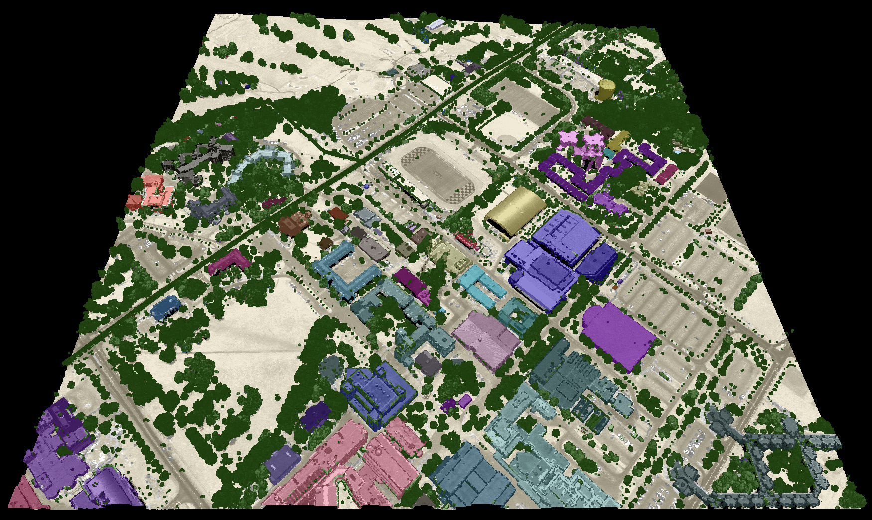
ClassifyBuildingsInLidar
This tool can be used to assign the building class (classification value 6) to all points within an
input LiDAR point cloud (--input) that are contained within the polygons of an input buildings
footprint vector (--buildings). The tool performs a simple point-in-polygon operation to determine
membership. The two inputs (i.e. the LAS file and vector) must share the same map projection. Furthermore,
any error in the definition of the building footprints will result in misclassified points in the output
LAS file (--output). In particular, if the footprints extend slightly beyond the actual building,
ground points situated adjacent to the building will be incorrectly classified. Thus, care must be
taken in digitizing building footprint polygons. Furthermore, where there are tall trees that overlap
significantly with the building footprint, these vegetation points will also be incorrectly assigned the
building class value.
See Also: FilterLidarClasses, LidarGroundPointFilter, ClipLidarToPolygon
Parameters:
| Flag | Description |
|---|---|
| -i, --input | Input LiDAR file |
| --buildings | Input vector polygons file |
| -o, --output | Output LiDAR file |
Python function:
wbt.classify_buildings_in_lidar(
    i,
    buildings,
    output,
    callback=default_callback
)
Command-line Interface:
>>./whitebox_tools -r=ClassifyBuildingsInLidar -v ^
--wd="/path/to/data/" -i='data.las' --polygons='lakes.shp' ^
-o='output.las'
Author: Dr. John Lindsay
Created: 17/11/2019
Last Modified: 17/11/2019
ClassifyLidar
Note this tool is part of a WhiteboxTools extension product. Please contact Whitebox Geospatial Inc. for information about purchasing a license activation key (https://www.whiteboxgeo.com/extension-pricing/).
This tool provides a basic classification of a LiDAR point cloud into ground, building, and vegetation classes. The algorithm performs the classification based on point neighbourhood geometric properties, including planarity, linearity, and height above the ground. There is also a point segmentation involved in the classification process.

The user may specify the names of the input and output LiDAR files (--input and --output).
Note that if the user does not specify the optional input/output LiDAR files, the tool will search for all
valid LiDAR (*.las, *.laz, *.zlidar) files contained within the current working directory. This feature can be useful
for processing a large number of LiDAR files in batch mode. When this batch mode is applied, the output file
names will be the same as the input file names but with a '_classified' suffix added to the end.
The search distance (--radius), defining the radius of the neighbourhood window surrounding each point, must
also be specified. If this parameter is set to a value that is too large, areas of high surface curvature on the
ground surface will be left unclassed and smaller buildings, e.g. sheds, will not be identified. If the parameter is
set too small, areas of low point density may provide unsatisfactory classification values. The larger this search
distance is, the longer the algorithm will take to processs a data set. For many airborne LiDAR data sets, a value
between 1.0 - 3.0 meters is likely appropriate.
The ground threshold parameter (--grd_threshold) determines how far above the tophat-transformed
surface a point must be to be excluded from the ground surface. This parameter also determines the maximum distance
a point can be from a plane or line model fit to a neighbourhood of points to be considered part of the model
geometry. Similarly the off-terrain object threshold parameter (--oto_threshold) is used to determine how high
above the ground surface a point must be to be considered either a vegetation or building point. The ground threshold
must be smaller than the off-terrain object threshold. If you find that breaks-in-slope in areas of more complex
ground topography are left unclassed (class = 1), this can be addressed by raising the ground threshold parameter.
The planarity and linearity thresholds (--planarity_threshold and --linearity_threshold) describe the minimum proportion
(0-1) of neighbouring points that must be part of a fitted model before the point is considered to be planar or linear.
Both of these properties are used by the algorithm in a variety of ways to determine final class values. Planar and
linear models are fit using a RANSAC-like algorithm, with the
main user-specified parameter of the number of iterations (--iterations). The larger the number of iterations the greater
the processing time will be.
The facade threshold (--facade_threshold) is the last user-specified parameter, and determines the maximum horizontal distance
that a point beneath a rooftop edge point may be to be considered part of the building facade (i.e. walls). The default
value is 0.5 m, although this value will depend on a number of factors, such as whether or not the building has balconies.
The algorithm generally does very well to identify deciduous (broad-leaf) trees but can at times struggle with incorrectly classifying dense coniferous (needle-leaf) trees as buildings. When this is the case, you may counter this tendency by lowering the planarity threshold parameter value. Similarly, the algorithm will generally leave overhead power lines as unclassified (class = 1), howevever, if you find that the algorithm misclassifies most such points as high vegetation (class = 5), this can be countered by lowering the linearity threshold value.
Note that if the input file already contains class data, these data will be overwritten in the output file.
See Also: ColourizeBasedOnClass, FilterLidar, ModifyLidar, SortLidar, SplitLidar
Parameters:
| Flag | Description |
|---|---|
| -i, --input | Name of the input LiDAR points |
| -o, --output | Name of the output LiDAR points |
| --radius | Search distance used in neighbourhood search (metres) |
| --grd_threshold | Ground threshold (metres) |
| --oto_threshold | Off-terrain object threshold (metres) |
| --planarity_threshold | Planarity threshold (0-1) |
| --linearity_threshold | Linearity threshold (0-1) |
| --iterations | Number of iterations |
| --facade_threshold | Facade threshold (metres) |
Python function:
wbt.classify_lidar(
    i=None,
    output=None,
    radius=1.5,
    grd_threshold=0.1,
    oto_threshold=2.0,
    planarity_threshold=0.85,
    linearity_threshold=0.70,
    iterations=30,
    facade_threshold=0.5,
    callback=default_callback
)
Command-line Interface:
>> ./whitebox_tools -r=ClassifyLidar -i=input.las ^
-o=output.las --radius=2.0 --grd_threshold=0.2 ^
--oto_threshold=1.0 --planarity_threshold=0.6 ^
--linearity_threshold=0.5 --iterations=50 ^
--facade_threshold=0.75
Source code is unavailable due to proprietary license.
Author: Whitebox Geospatial Inc. (c)
Created: 18/02/2022
Last Modified: 25/02/2022
ClassifyOverlapPoints
This tool can be used to flag points within an input LiDAR file (--input) that overlap with other
nearby points from different flightlines, i.e. to identify overlap points. The flightline associated
with a LiDAR point is assumed to be contained within the point's Point Source ID (PSID) property.
If the PSID property is not set, or has been lost, users may with to apply the RecoverFlightlineInfo
tool prior to running FlightlineOverlap.
Areas of multiple flightline overlap tend to have point densities that are far greater than areas of single flightlines. This can produce suboptimal results for applications that assume regular point distribution, e.g. in point classification operations.
The tool works by applying a square grid over the extent of the input LiDAR file. The grid cell size is
determined by the user-defined --resolution parameter. Grid cells containing multiple PSIDs, i.e.
with more than one flightline, are then identified. Overlap points within these grid cells can then be
flagged on the basis of a user-defined --criterion. The flagging options include the following:
| Criterion | Overlap Point Definition |
|---|---|
max scan angle | All points that share the PSID of the point with the maximum absolute scan angle |
not min point source ID | All points with a different PSID to that of the point with the lowest PSID |
not min time | All points with a different PSID to that of the point with the minimum GPS time |
multiple point source IDs | All points in grid cells with multiple PSIDs, i.e. all overlap points. |
Note that the max scan angle criterion may not be appropriate when more than two flightlines overlap,
since it will result in only flagging points from one of the multiple flightlines.
It is important to set the --resolution parameter appropriately, as setting this value too high will
yield the filtering of points in non-overlap areas, and setting the resolution to low will result in
fewer than expected points being flagged. An appropriate resolution size value may require experimentation,
however a value that is 2-3 times the nominal point spacing has been previously recommended. The nominal
point spacing can be determined using the LidarInfo tool.
By default, all flagged overlap points are reclassified in the output LiDAR file (--output) to class
12. Alternatively, if the user specifies the --filter parameter, then each overlap point will be
excluded from the output file. Classified overlap points may also be filtered from LiDAR point clouds
using the FilterLidar tool.
Note that this tool is intended to be applied to LiDAR tile data containing points that have been merged from multiple overlapping flightlines. It is commonly the case that airborne LiDAR data from each of the flightlines from a survey are merged and then tiled into 1 km2 tiles, which are the target dataset for this tool.
See Also: FlightlineOverlap, RecoverFlightlineInfo, FilterLidar, LidarInfo
Parameters:
| Flag | Description |
|---|---|
| -i, --input | Input LiDAR file |
| -o, --output | Output LiDAR file |
| --resolution | The size of the square area used to evaluate nearby points in the LiDAR data |
| -c, --criterion | Criterion used to identify overlapping points; options are 'max scan angle', 'not min point source ID', 'not min time', 'multiple point source IDs' |
| --filter | Filter out points from overlapping flightlines? If false, overlaps will simply be classified |
Python function:
wbt.classify_overlap_points(
    i,
    output,
    resolution=2.0,
    criterion="max scan angle",
    filter=False,
    callback=default_callback
)
Command-line Interface:
>>./whitebox_tools -r=ClassifyOverlapPoints -v ^
--wd="/path/to/data/" -i=file.las -o=outfile.las ^
--resolution=2.0
Author: Dr. John Lindsay
Created: 27/04/2018
Last Modified: 24/03/2022
ClipLidarToPolygon
This tool can be used to isolate, or clip, all of the LiDAR points in a LAS file (--input) contained within
one or more vector polygon features. The user must specify the name of the input clip file (--polygons), which
must be a vector of a Polygon base shape type. The clip file may contain multiple polygon features and polygon hole
parts will be respected during clipping, i.e. LiDAR points within polygon holes will be removed from the output LAS
file.
Use the ErasePolygonFromLidar tool to perform the complementary operation of removing points from a LAS file that are contained within a set of polygons.
See Also: ErasePolygonFromLidar, FilterLidar, Clip, ClipRasterToPolygon
Parameters:
| Flag | Description |
|---|---|
| -i, --input | Input LiDAR file |
| --polygons | Input vector polygons file |
| -o, --output | Output LiDAR file |
Python function:
wbt.clip_lidar_to_polygon(
    i,
    polygons,
    output,
    callback=default_callback
)
Command-line Interface:
>>./whitebox_tools -r=ClipLidarToPolygon -v ^
--wd="/path/to/data/" -i='data.las' --polygons='lakes.shp' ^
-o='output.las'
Author: Dr. John Lindsay
Created: 25/04/2018
Last Modified: 26/07/2019
ColourizeBasedOnClass
Note this tool is part of a WhiteboxTools extension product. Please contact Whitebox Geospatial Inc. for information about purchasing a license activation key (https://www.whiteboxgeo.com/extension-pricing/).
This tools sets the RGB colour values of an input LiDAR point cloud (--input) based on the point classifications.
Rendering a point cloud in this way can aid with the determination of point classification accuracy, by allowing
you to determine if there are certain areas within a LiDAR tile, or certain classes, that are problematic during
the point classification process.
By default, the tool renders buildings in red (see table below). However, the tool also provides the option to
render each building in a unique colour (--use_unique_clrs_for_buildings), providing a visually stunning
LiDAR-based map of built-up areas. When this option is selected, the user must also specify the --radius
parameter, which determines the search distance used during the building segmentation operation. The --radius
parameter is optional, and if unspecified (when the --use_unique_clrs_for_buildings flag is used), a value of
2.0 will be used.
The specific colours used to render each point class can optionally be set by the user with the --clr_str parameter.
The value of this parameter may list specific class values (0-18) and corresponding colour values in either a
red-green-blue (RGB) colour triplet form (i.e. (r, g, b)), or or a hex-colour, of either form #e6d6aa or
0xe6d6aa (note the # and 0x prefixes used to indicate hexadecimal numbers; also either lowercase or
capital letter values are acceptable). The following is an example of the a valid --clr_str that sets the
ground (class 2) and high vegetation (class 5) colours used for rendering:
2: (184, 167, 108); 5: #9ab86c
Notice that 1) each class is separated by a semicolon (';'), 2) class values and colour values are separated by colons (':'), and 3) either RGB and hex-colour forms are valid.
If a --clr_str parameter is not provided, the tool will use the default colours used for each class (see table below).
Class values are assumed to follow the class designations listed in the LAS specification:
| Classification Value | Meaning | Default Colour |
|---|---|---|
| 0 | Created never classified | |
| 1 | Unclassified | |
| 2 | Ground | |
| 3 | Low Vegetation | |
| 4 | Medium Vegetation | |
| 5 | High Vegetation | |
| 6 | Building | |
| 7 | Low Point (noise) | |
| 8 | Reserved | |
| 9 | Water | |
| 10 | Rail | |
| 11 | Road Surface | |
| 12 | Reserved | |
| 13 | Wire – Guard (Shield) | |
| 14 | Wire – Conductor (Phase) | |
| 15 | Transmission Tower | |
| 16 | Wire-structure Connector (e.g. Insulator) | |
| 17 | Bridge Deck | |
| 18 | High noise |
The point RGB colour values can be blended with the intensity data to create a particularly effective
visualization, further enhancing the visual interpretation of point return properties. The --intensity_blending
parameter value, which must range from 0% (no intensity blending) to 100% (all intensity), is used to
set the degree of intensity/RGB blending.
Because the output file contains RGB colour data, it is possible that it will be larger than the input file. If the input file does contain valid RGB data, the output will be similarly sized, but the input colour data will be replaced in the output file with the point-return colours.
The output file can be visualized using any point cloud renderer capable of displaying point RGB information. We recommend the plas.io LiDAR renderer but many similar open-source options exist.
See Also: ColourizeBasedOnPointReturns, LidarColourize
Parameters:
| Flag | Description |
|---|---|
| -i, --input | Name of the input LiDAR points |
| -o, --output | Name of the output LiDAR points |
| --intensity_blending | Intensity blending amount (0-100%) |
| --clr_str | Colour values, e.g. 2: (184, 167, 108); 5: #9ab86c |
| --use_unique_clrs_for_buildings | Use unique colours for each building? |
| --radius | Search distance used in neighbourhood search |
Python function:
wbt.colourize_based_on_class(
    i=None,
    output=None,
    intensity_blending=50.0,
    clr_str="",
    use_unique_clrs_for_buildings=False,
    radius="",
    callback=default_callback
)
Command-line Interface:
>> ./whitebox_tools -r=ColourizeBasedOnClass -i=input.las ^
-o=output.las --clr_str='2: (184, 167, 108); 5: (100, 255, 50)' ^
--use_unique_clrs_for_buildings --radius=2.5
Source code is unavailable due to proprietary license.
Author: Whitebox Geospatial Inc. (c)
Created: 09/04/2022
Last Modified: 10/04/2022
ColourizeBasedOnPointReturns
Note this tool is part of a WhiteboxTools extension product. Please contact Whitebox Geospatial Inc. for information about purchasing a license activation key (https://www.whiteboxgeo.com/extension-pricing/).
This tool sets the RGB colour values of a LiDAR point cloud (--input) based on the point returns. It specifically
renders only-return, first-return, intermediate-return, and last-return points in different colours, storing
these data in the RGB colour data of the output LiDAR file (--output). Colourizing the points in a LiDAR
point cloud based on return properties can aid with the visual inspection of point distributions, and therefore,
the quality assurance/quality control (QA/QC) of LiDAR data tiles. For example, this visualization process can
help to determine if there are areas of vegetation where there is insufficient coverage of ground points,
perhaps due to acquisition of the data during leaf-on conditions. There is often an assumption in LiDAR data
processing that the ground surface can be modelled using a subset of the only-return and last-return points
(beige and blue in the image below). However, under heavy forest cover, and in particular if the data were
collected during leaf-on conditions or if there is significant coverage of conifer trees, the only-return
and last-return points may be poor approximations of the ground surface. This tool can help to determine the
extent to which this is the case for a particular data set.

The specific colours used to render each return type can be set by the user with the --only, --first,
--intermediate, and --last parameters. Each parameter takes either a red-green-blue (RGB) colour triplet,
of the form (r,g,b), or a hex-colour, of either form #e6d6aa or 0xe6d6aa (note the # and 0x prefixes
used to indicate hexadecimal numbers; also either lowercase or capital letter values are acceptable).
The point RGB colour values can be blended with the intensity data to create a particularly effective
visualization, further enhancing the visual interpretation of point return properties. The --intensity_blending
parameter value, which must range from 0% (no intensity blending) to 100% (all intensity), is used to
set the degree of intensity/RGB blending.
Because the output file contains RGB colour data, it is possible that it will be larger than the input file. If the input file does contain valid RGB data, the output will be similarly sized, but the input colour data will be replaced in the output file with the point-return colours.
The output file can be visualized using any point cloud renderer capable of displaying point RGB information. We recommend the plas.io LiDAR renderer but many similar open-source options exist.
This tool is a convenience function and can alternatively be achieved using the ModifyLidar tool with the statement:
rgb=if(is_only, (230,214,170), if(is_last, (0,0,255), if(is_first, (0,255,0), (255,0,255))))
The ColourizeBasedOnPointReturns tool is however significantly faster for this operation than the ModifyLidar tool because the expression above must be executed dynamically for each point.
See Also: ModifyLidar, LidarColourize
Parameters:
| Flag | Description |
|---|---|
| -i, --input | Name of the input LiDAR points |
| -o, --output | Name of the output LiDAR points |
| --intensity_blending | Intensity blending amount (0-100%) |
| --only | Only return colour, e.g. (230,214,170), #e6d6aa, or 0xe6d6aa |
| --first | First return colour, e.g. (230,214,170), #e6d6aa, or 0xe6d6aa |
| --intermediate | Intermediate return colour, e.g. (230,214,170), #e6d6aa, or 0xe6d6aa |
| --last | Last return colour, e.g. (230,214,170), #e6d6aa, or 0xe6d6aa |
Python function:
wbt.colourize_based_on_point_returns(
    i=None,
    output=None,
    intensity_blending=50.0,
    only="(230,214,170)",
    first="(0,140,0)",
    intermediate="(255,0,255)",
    last="(0,0,255)",
    callback=default_callback
)
Command-line Interface:
>> ./whitebox_tools -r=ColourizeBasedOnPointReturns ^
-i=input.las -o=output.las
Source code is unavailable due to proprietary license.
Author: Whitebox Geospatial Inc. (c)
Created: 03/04/2022
Last Modified: 10/04/2022
ErasePolygonFromLidar
This tool can be used to remove, or erase, all of the LiDAR points in a LAS file (--input) contained within
one or more vector polygon features. The user must specify the name of the input clip file (--polygons), which
must be a vector of a Polygon base shape type. The clip file may contain multiple polygon features and polygon hole
parts will be respected during clipping, i.e. LiDAR points within polygon holes will be remain in the output LAS
file.
Use the ClipLidarToPolygon tool to perform the complementary operation of clipping (isolating) points from a LAS file that are contained within a set of polygons, while removing points that lie outside the input polygons.
See Also: ClipLidarToPolygon, FilterLidar, Clip, ClipRasterToPolygon
Parameters:
| Flag | Description |
|---|---|
| -i, --input | Input LiDAR file |
| --polygons | Input vector polygons file |
| -o, --output | Output LiDAR file |
Python function:
wbt.erase_polygon_from_lidar(
    i,
    polygons,
    output,
    callback=default_callback
)
Command-line Interface:
>>./whitebox_tools -r=ErasePolygonFromLidar -v ^
--wd="/path/to/data/" -i='data.las' --polygons='lakes.shp' ^
-o='output.las'
Author: Dr. John Lindsay
Created: 25/04/2018
Last Modified: 12/10/2018
FilterLidar
Note this tool is part of a WhiteboxTools extension product. Please visit Whitebox Geospatial Inc. for information about purchasing a license activation key (https://www.whiteboxgeo.com/extension-pricing/).
The FilterLidar tool is a very powerful tool for filtering points within a LiDAR point cloud based on point
properties. Complex filter statements (--statement) can be used to include or exclude points in the
output file (--output).
Note that if the user does not specify the optional input LiDAR file (--input), the tool will search for all
valid LiDAR (*.las, *.laz, *.zlidar) files contained within the current working directory. This feature can be useful
for processing a large number of LiDAR files in batch mode. When this batch mode is applied, the output file
names will be the same as the input file names but with a '_filtered' suffix added to the end.
Points are either included or excluded from the output file by creating conditional filter statements. Statements must be valid Rust syntax and evaluate to a Boolean. Any of the following variables are acceptable within the filter statement:
| Variable Name | Description |
|---|---|
| x | The point x coordinate |
| y | The point y coordinate |
| z | The point z coordinate |
| intensity | The point intensity value |
| ret | The point return number |
| nret | The point number of returns |
| is_only | True if the point is an only return (i.e. ret == nret == 1), otherwise false |
| is_multiple | True if the point is a multiple return (i.e. nret > 1), otherwise false |
| is_early | True if the point is an early return (i.e. ret == 1), otherwise false |
| is_intermediate | True if the point is an intermediate return (i.e. ret > 1 && ret < nret), otherwise false |
| is_late | True if the point is a late return (i.e. ret == nret), otherwise false |
| is_first | True if the point is a first return (i.e. ret == 1 && nret > 1), otherwise false |
| is_last | True if the point is a last return (i.e. ret == nret && nret > 1), otherwise false |
| class | The class value in numeric form, e.g. 0 = Never classified, 1 = Unclassified, 2 = Ground, etc. |
| is_noise | True if the point is classified noise (i.e. class == 7 |
| is_synthetic | True if the point is synthetic, otherwise false |
| is_keypoint | True if the point is a keypoint, otherwise false |
| is_withheld | True if the point is withheld, otherwise false |
| is_overlap | True if the point is an overlap point, otherwise false |
| scan_angle | The point scan angle |
| scan_direction | True if the scanner is moving from the left towards the right, otherwise false |
| is_flightline_edge | True if the point is situated along the filightline edge, otherwise false |
| user_data | The point user data |
| point_source_id | The point source ID |
| scanner_channel | The point scanner channel |
| time | The point GPS time, if it exists, otherwise 0 |
| red | The point red value, if it exists, otherwise 0 |
| green | The point green value, if it exists, otherwise 0 |
| blue | The point blue value, if it exists, otherwise 0 |
| nir | The point near infrared value, if it exists, otherwise 0 |
| pt_num | The point number within the input file |
| n_pts | The number of points within the file |
| min_x | The file minimum x value |
| mid_x | The file mid-point x value |
| max_x | The file maximum x value |
| min_y | The file minimum y value |
| mid_y | The file mid-point y value |
| max_y | The file maximum y value |
| min_z | The file minimum z value |
| mid_z | The file mid-point z value |
| max_z | The file maximum z value |
| dist_to_pt | The distance from the point to a specified xy or xyz point, e.g. dist_to_pt(562500, 4819500) or dist_to_pt(562500, 4819500, 320) |
| dist_to_line | The distance from the point to the line passing through two xy points, e.g. dist_to_line(562600, 4819500, 562750, 4819750) |
| dist_to_line_seg | The distance from the point to the line segment defined by two xy end-points, e.g. dist_to_line_seg(562600, 4819500, 562750, 4819750) |
| within_rect | 1 if the point falls within the bounds of a 2D or 3D rectangle, otherwise 0. Bounds are defined as within_rect(ULX, ULY, LRX, LRY) or within_rect(ULX, ULY, ULZ, LRX, LRY, LRZ) |
In addition to the point properties defined above, if the user applies the LidarEigenvalueFeatures
tool on the input LiDAR file, the FilterLidar tool will automatically read in the additional *.eigen
file, which include the eigenvalue-based point neighbourhood measures, such as lambda1, lambda2, lambda3,
linearity, planarity, sphericity, omnivariance, eigentropy, slope, and residual. See the
LidarEigenvalueFeatures documentation for details on each of these metrics describing the structure
and distribution of points within the neighbourhood surrounding each point in the LiDAR file.
Statements can be as simple or complex as desired. For example, to filter out all points that are classified noise (i.e. class numbers 7 or 18):
!is_noise
The following is a statement to retain only the late returns from the input file (i.e. both last and single returns):
ret == nret
Notice that equality uses the == symbol an inequality uses the != symbol. As an equivalent to the above
statement, we could have used the is_late point property:
is_late
If we want to remove all points outside of a range of xy values:
x >= 562000 && x <= 562500 && y >= 4819000 && y <= 4819500
Notice how we can combine multiple constraints using the && (logical AND) and || (logical OR) operators.
As an alternative to the above statement, we could have used the within_rect function:
within_rect(562000, 4819500, 562500, 4819000)
If we want instead to exclude all of the points within this defined region, rather than to retain them, we
simply use the ! (logial NOT):
!(x >= 562000 && x <= 562500 && y >= 4819000 && y <= 4819500)
or, simply:
!within_rect(562000, 4819500, 562500, 4819000)
If we need to find all of the ground points within 150 m of (562000, 4819500), we could use:
class == 2 && dist_to_pt(562000, 4819500) <= 150.0
The following statement outputs all non-vegetation classed points in the upper-right quadrant:
!(class == 3 && class != 4 && class != 5) && x < min_x + (max_x - min_x) / 2.0 && y > max_y - (max_y - min_y) / 2.0
As demonstrated above, the FilterLidar tool provides an extremely flexible, powerful, and easy means for retaining and removing points from point clouds based on any of the common LiDAR point attributes.
See Also: FilterLidarClasses, FilterLidarScanAngles, ModifyLidar, ErasePolygonFromLidar, ClipLidarToPolygon, SortLidar, LidarEigenvalueFeatures
Parameters:
| Flag | Description |
|---|---|
| -i, --input | Name of the input LiDAR points |
| -o, --output | Name of the output LiDAR points |
| -s, --statement | Filter statement e.g. x < 5000.0 && y > 100.0 && is_late && !is_noise. This statement must be a valid Rust statement |
Python function:
wbt.filter_lidar(
    i=None,
    output=None,
    statement="",
    callback=default_callback
)
Command-line Interface:
>> ./whitebox_tools -r=FilterLidar -i=input.las -o=output.las ^
--statement="x<5000.0 && y>100.0"
Source code is unavailable due to proprietary license.
Author: Whitebox Geospatial Inc. (c)
Created: 05/02/2022
Last Modified: 05/02/2022
FilterLidarClasses
This tool can be used to remove points within a LAS LiDAR file that possess certain
specified class values. The user must input the names of the input (--input) and
output (--output) LAS files and the class values to be excluded (--exclude_cls).
Class values are specified by their numerical values, such that:
| Classification Value | Meaning |
|---|---|
| 0 | Created never classified |
| 1 | Unclassified |
| 2 | Ground |
| 3 | Low Vegetation |
| 4 | Medium Vegetation |
| 5 | High Vegetation |
| 6 | Building |
| 7 | Low Point (noise) |
| 8 | Reserved |
| 9 | Water |
| 10 | Rail |
| 11 | Road Surface |
| 12 | Reserved |
| 13 | Wire – Guard (Shield) |
| 14 | Wire – Conductor (Phase) |
| 15 | Transmission Tower |
| 16 | Wire-structure Connector (e.g. Insulator) |
| 17 | Bridge Deck |
| 18 | High noise |
Thus, to filter out low and high noise points from a point cloud, specify
--exclude_cls='7,18'. Class ranges may also be specified, e.g. --exclude_cls='3-5,7,18'.
Notice that usage of this tool assumes that the
LAS file has underwent a comprehensive point classification, which not all
point clouds have had. Use the LidarInfo tool determine the distribution
of various class values in your file.
See Also: LidarInfo
Parameters:
| Flag | Description |
|---|---|
| -i, --input | Input LiDAR file |
| -o, --output | Output LiDAR file |
| --exclude_cls | Optional exclude classes from interpolation; Valid class values range from 0 to 18, based on LAS specifications. Example, --exclude_cls='3,4,5,6,7,18' |
Python function:
wbt.filter_lidar_classes(
    i,
    output,
    exclude_cls=None,
    callback=default_callback
)
Command-line Interface:
>>./whitebox_tools -r=FilterLidarClasses -v ^
--wd="/path/to/data/" -i="input.las" -o="output.las" ^
--exclude_cls='7,18'
Author: Dr. John Lindsay
Created: 24/07/2019
Last Modified: 16/01/2020
FilterLidarScanAngles
Removes points in a LAS file with scan angles greater than a threshold.
Parameters:
| Flag | Description |
|---|---|
| -i, --input | Input LiDAR file |
| -o, --output | Output LiDAR file |
| --threshold | Scan angle threshold |
Python function:
wbt.filter_lidar_scan_angles(
    i,
    output,
    threshold,
    callback=default_callback
)
Command-line Interface:
>>./whitebox_tools -r=FilterLidarScanAngles -v ^
--wd="/path/to/data/" -i="input.las" -o="output.las" ^
--threshold=10.0
Author: Dr. John Lindsay
Created: September 17, 2017
Last Modified: 12/10/2018
FindFlightlineEdgePoints
Identifies points along a flightline's edge in a LAS file.
Parameters:
| Flag | Description |
|---|---|
| -i, --input | Input LiDAR file |
| -o, --output | Output file |
Python function:
wbt.find_flightline_edge_points(
    i,
    output,
    callback=default_callback
)
Command-line Interface:
>>./whitebox_tools -r=FindFlightlineEdgePoints -v ^
--wd="/path/to/data/" -i="input.las" -o="output.las"
Author: Dr. John Lindsay
Created: June 14, 2017
Last Modified: 12/10/2018
FlightlineOverlap
This tool can be used to map areas of overlapping flightlines in an input LiDAR (LAS) file (--input).
The output raster file (--output) will contain the number of different flightlines that are contained
within each grid cell. The user must specify the desired cell size (--resolution). The flightline
associated with a LiDAR point is assumed to be contained within the point's Point Source ID property.
Thus, the tool essentially counts the number of different Point Source ID values among the points contained
within each grid cell. If the Point Source ID property is not set, or has been lost, users may with to
apply the RecoverFlightlineInfo tool prior to running FlightlineOverlap.
It is important to set the --resolution parameter appropriately, as setting this value too high will
yield the mis-characterization of non-overlap areas, and setting the resolution to low will result in
fewer than expected overlap areas. An appropriate resolution size value may require experimentation,
however a value that is 2-3 times the nominal point spacing has been previously recommended. The nominal
point spacing can be determined using the LidarInfo tool.
Note that this tool is intended to be applied to LiDAR tile data containing points that have been merged from multiple overlapping flightlines. It is commonly the case that airborne LiDAR data from each of the flightlines from a survey are merged and then tiled into 1 km2 tiles, which are the target dataset for this tool.
Like many of the LiDAR related tools, the input and output file parameters are optional. If left unspecified, the tool will locate all valid LiDAR files within the current Whitebox working directory and use these for calculation (specifying the output raster file name based on the associated input LiDAR file). This can be a helpful way to run the tool on a batch of user inputs within a specific directory.
See Also: ClassifyOverlapPoints, RecoverFlightlineInfo, LidarInfo
Parameters:
| Flag | Description |
|---|---|
| -i, --input | Input LiDAR file |
| -o, --output | Output file |
| --resolution | Output raster's grid resolution |
Python function:
wbt.flightline_overlap(
    i=None,
    output=None,
    resolution=1.0,
    callback=default_callback
)
Command-line Interface:
>>./whitebox_tools -r=FlightlineOverlap -v ^
--wd="/path/to/data/" -i=file.las -o=outfile.tif ^
--resolution=2.0"
./whitebox_tools -r=FlightlineOverlap -v ^
--wd="/path/to/data/" -i=file.las -o=outfile.tif ^
--resolution=5.0 --palette=light_quant.plt
Author: Dr. John Lindsay
Created: 19/06/2017
Last Modified: 24/03/2022
HeightAboveGround
This tool normalizes an input LiDAR point cloud (--input) such that point z-values in the output LAS file
(--output) are converted from elevations to heights above the ground, specifically the height above the
nearest ground-classified point. The input LAS file must have ground-classified points, otherwise the tool
will return an error. The LidarTophatTransform tool can be used to perform the normalization if a ground
classification is lacking.
See Also: LidarTophatTransform
Parameters:
| Flag | Description |
|---|---|
| -i, --input | Input LiDAR file (including extension) |
| -o, --output | Output lidar file (including extension) |
Python function:
wbt.height_above_ground(
    i=None,
    output=None,
    callback=default_callback
)
Command-line Interface:
>>./whitebox_tools -r=HeightAboveGround -v ^
--wd="/path/to/data/" -i=file.las -o=outfile.tif
Author: Dr. John Lindsay
Created: 08/11/2019
Last Modified: 15/12/2019
IndividualTreeDetection
This tool can be used to identify points in a LiDAR point cloud that are associated with the tops of individual trees. The
tool takes a LiDAR point cloud as an input (input_lidar) and it is best if the input file has been normalized using the
NormalizeLidar or LidarTophatTransform tools, such that points record height above the ground surface. Note that the input
parameter is optional and if left unspecified the tool will search for all valid LiDAR (*.las, *.laz, *.zlidar) files
contained within the current working directory. This 'batch mode' operation is common among many of the LiDAR processing
tools. Output vectors are saved to disc automatically for each processed LiDAR file when operating in batch mode.
The tool will evaluate the points within a local neighbourhood around each point in the input point cloud and determine
if it is the highest point within the neighbourhood. If a point is the highest local point, it will be entered into the
output vector file (output). The neighbourhood size can vary, with higher canopy positions generally associated with larger
neighbourhoods. The user specifies the min_search_radius and min_height parameters, which default to 1 m and 0 m
respectively. If the min_height parameter is greater than zero, all points that are less than this value above the
ground (assuming the input point cloud measures this height parameter) are ignored, which can be a useful mechanism
for removing shorter trees and other vegetation from the analysis. If the user specifies the max_search_radius and
max_height parameters, the search radius will be determined by linearly interpolation based on point height and the
min/max search radius and height parameter values. Points that are above the max_height parameter will be processed
with search neighbourhoods sized max_search_radius. If the max radius and height parameters are unspecified, they
are set to the same values as the minimum radius and height parameters, i.e., the neighbourhood size does not increase
with canopy height.
If the point cloud contains point classifications, it may be useful to exclude all non-vegetation points. To do this
simply set the only_use_veg parameter to True. This parameter should only be set to True when you know that the
input file contains point classifications, otherwise the tool may generate an empty output vector file.
See Also: NormalizeLidar, LidarTophatTransform
Parameters:
| Flag | Description |
|---|---|
| -i, --input | Name of the input LiDAR file |
| -o, --output | Name of the output vector points file |
| --min_search_radius | Minimum search radius (m) |
| --min_height | Minimum height (m) |
| --max_search_radius | Maximum search radius (m) |
| --max_height | Maximum height (m) |
| --only_use_veg | Only use veg. class points? |
Python function:
wbt.individual_tree_detection(
    i=None,
    output=None,
    min_search_radius=1.0,
    min_height=0.0,
    max_search_radius="",
    max_height="",
    only_use_veg=False,
    callback=default_callback
)
Command-line Interface:
>> ./whitebox_tools -r=IndividualTreeDetection -i=points.laz ^
-o=tree_tops.shp --min_search_radius=1.5 --min_height=2.0 ^
--max_search_radius=8.0 --max_height=30.0 --only_use_veg
Source code is unavailable due to proprietary license.
Author: Dr. John Lindsay
Created: 05/03/2023
Last Modified: 05/03/2023
LasToAscii
This tool can be used to convert one or more LAS file, containing LiDAR data, into ASCII files. The user must
specify the name(s) of the input LAS file(s) (--inputs). Each input file will have a correspondingly named
output file with a .csv file extension. CSV files are comma separated value files and contain tabular data
with each column corresponding to a field in the table and each row a point value. Fields are separated by
commas in the ASCII formatted file. The output point data, each on a separate line, will take the format:
X,Y,Z,INTENSITY,CLASS,RETURN,NUM_RETURN,SCAN_ANGLE
If the LAS file has a point format that contains RGB data, the final three columns will contain the RED, GREEN, and BLUE values respectively. Use the AsciiToLas tool to convert a text file containing LiDAR point data into a LAS file.
See Also: AsciiToLas
Parameters:
| Flag | Description |
|---|---|
| -i, --inputs | Input LiDAR files |
Python function:
wbt.las_to_ascii(
    inputs,
    callback=default_callback
)
Command-line Interface:
>>./whitebox_tools -r=LasToAscii -v --wd="/path/to/data/" ^
-i="file1.las, file2.las, file3.las"
Author: Dr. John Lindsay
Created: 16/07/2017
Last Modified: 29/02/2020
LasToLaz
Note this tool is part of a WhiteboxTools extension product. Please visit Whitebox Geospatial Inc. for information about purchasing a license activation key (https://www.whiteboxgeo.com/extension-pricing/).
This tool converts one or more LiDAR files in the uncompressed
LAS format into a compressed
LAZ file. Both the --input and --output parameters are optional. If these
parameters are not specified by the user, the tool will search for all LAS files contained within the
current WhiteboxTools working directory. This feature can be useful when you need to convert a large
number of LAS files. This batch processing mode enables the tool to perform parallel data processing,
which can significantly improve the efficiency of data conversion for datasets with many LiDAR tiles.
When run in this batch mode, the output file (--output) also need not be specified; the tool will
instead create an output file with the same name as each input LiDAR file, but with the .laz extension.
The LAZ encoder/decoder that is used by the LasToLaz tool is not necessarily faster than other LAZ
libraries, such as the common laszip LiDAR conversion utility program. While single-tile conversion
performance is likely to be on par or slighly slower than laszip, the parallelization of the LazToLas
tool when run in batch mode can result in significant performance gains in applications working on many
individual LAS tiles. The following table shows a comparison of the performance of the LasToLaz tool
with laszip (time laszip -i *.las) for a number of sample data sets. All tests were performed on a
2013 MacPro with an 8-core 3.0 GHz Intel Xeon processor with 64 GB memory. Files were written to an
external hard drive, and times are inclusive of file I/O.
| Dataset Name | Num. Tiles | laszip | LasToLaz |
|---|---|---|---|
| Guelph | 201 | 1481.0s | 616.8s |
| Broughtons's Creek | 331 | 139.3s | 48.6s |
| Big Otter Creek | 1089 | 5115.2s | 2689.7s |
| Ottawa 2015 | 661 | 3308.3s | 1139.9s |
See Also: LazToLas, LasToZlidar, ZlidarToLas, LasToAscii, LasToShapefile
Parameters:
| Flag | Description |
|---|---|
| -i, --input | Name of the input LAS files (leave blank to use all LAS files in WorkingDirectory |
| -o, --output | Output LAZ file (including extension) |
Python function:
wbt.las_to_laz(
    i=None,
    output=None,
    callback=default_callback
)
Command-line Interface:
>> ./whitebox_tools -r=LazToLas -i=file.laz -o=outfile.las
Source code is unavailable due to proprietary license.
Author: Whitebox Geospatial Inc. (c)
Created: 15/06/2021
Last Modified: 15/06/2021
LasToMultipointShapefile
Converts one or more LAS files into MultipointZ vector Shapefiles. When the input parameter is not specified, the tool grids all LAS files contained within the working directory.
This tool can be used in place of the LasToShapefile tool when the number of points are relatively high and when the desire is to represent the x,y,z position of points only. The z values of LAS points will be stored in the z-array of the output Shapefile. Notice that because the output file stores each point in a single multi-point record, this Shapefile representation, while unable to represent individual point classes, return numbers, etc, is an efficient means of converting LAS point positional information.
See Also: LasToShapefile
Parameters:
| Flag | Description |
|---|---|
| -i, --input | Input LiDAR file |
Python function:
wbt.las_to_multipoint_shapefile(
    i=None,
    callback=default_callback
)
Command-line Interface:
>>./whitebox_tools -r=LasToMultipointShapefile -v ^
--wd="/path/to/data/" -i=input.las
Author: Dr. John Lindsay
Created: 04/09/2018
Last Modified: 19/05/2020
LasToShapefile
This tool converts one or more LAS files into a POINT vector. When the input parameter is not specified, the tool grids all LAS files contained within the working directory. The attribute table of the output Shapefile will contain fields for the z-value, intensity, point class, return number, and number of return.
This tool can be used in place of the LasToMultipointShapefile tool when the number of points are relatively low and when the desire is to represent more than simply the x,y,z position of points. Notice however that because each point in the input LAS file will be represented as a separate record in the output Shapefile, the output file will be many time larger than the equivalent output of the LasToMultipointShapefile tool. There is also a practical limit on the total number of records that can be held in a single Shapefile and large LAS files approach this limit. In these cases, the LasToMultipointShapefile tool should be preferred instead.
See Also: LasToMultipointShapefile
Parameters:
| Flag | Description |
|---|---|
| -i, --input | Input LiDAR file |
Python function:
wbt.las_to_shapefile(
    i=None,
    callback=default_callback
)
Command-line Interface:
>>./whitebox_tools -r=LasToShapefile -v --wd="/path/to/data/" ^
-i=input.las
Author: Dr. John Lindsay
Created: 01/10/2018
Last Modified: 20/05/2020
LasToZlidar
This tool can be used to convert one or more LAS files into the
zLidar compressed
LiDAR data format. The tool takes a list of input LAS files (--inputs). If --inputs
is unspecified, the tool will use all LAS files contained within the working directory
as the tool inputs. The user may also specify an optional output directory --outdir.
If this parameter is unspecified, each output zLidar file will be written to the same
directory as the input files.
See Also: ZlidarToLas, LasToShapefile, LasToAscii
Parameters:
| Flag | Description |
|---|---|
| -i, --inputs | Input LAS files |
| --outdir | Output directory into which zlidar files are created. If unspecified, it is assumed to be the same as the inputs |
| --compress | Compression method, including 'brotli' and 'deflate' |
| --level | Compression level (1-9) |
Python function:
wbt.las_to_zlidar(
    inputs=None,
    outdir=None,
    compress="brotli",
    level=5,
    callback=default_callback
)
Command-line Interface:
>>./whitebox_tools -r=LasToZlidar -v --wd="/path/to/data/" ^
-i="file1.las, file2.las, file3.las"
Author: Dr. John Lindsay
Created: 13/05/2020
Last Modified: 15/05/2020
LazToLas
Note this tool is part of a WhiteboxTools extension product. Please visit Whitebox Geospatial Inc. for information about purchasing a license activation key (https://www.whiteboxgeo.com/extension-pricing/).
This tool converts one or more LiDAR files in the compressed LAZ format into an
uncompressed LAS file. Both the
--input and --output parameters are optional. If these parameters are not specified by the user, the
tool will search for all LAZ files contained within the current WhiteboxTools working directory. This
feature can be useful when you need to convert a large number of LAZ files. This batch processing mode
enables the tool to perform parallel data processing, which can significantly improve the efficiency of
data conversion for datasets with many LiDAR tiles. When run in this batch mode, the output file
(--output) also need not be specified; the tool will instead create an output file with the same name
as each input LiDAR file, but with the .las extension.
The LAZ encoder/decoder that is used by the LazToLas tool is not necessarily faster than other LAZ
libraries, such as the common laszip LiDAR conversion utility program. While single-tile conversion
performance is likely to be on par or slighly slower than laszip, the parallelization of the LazToLas
tool when run in batch mode can result in significant performance gains in applications working on many
individual LAZ tiles. The following table shows a comparison of the performance of the LazToLas tool
with laszip (time laszip -i *.laz) for a number of sample data sets. All tests were performed on a
2013 MacPro with an 8-core 3.0 GHz Intel Xeon processor with 64 GB memory. Files were written to an
external hard drive, and times are inclusive of file I/O.
| Dataset Name | Num. Tiles | laszip | LazToLas |
|---|---|---|---|
| Guelph | 201 | 3062.3s | 525.9s |
| Broughtons's Creek | 331 | 261.4s | 53.2s |
| Big Otter Creek | 1089 | 7200.2s | 1923.9s |
| Ottawa 2015 | 661 | 6950.6s | 1130.5s |
See Also: LasToLaz, LasToZlidar, ZlidarToLas, LasToAscii, LasToShapefile
Parameters:
| Flag | Description |
|---|---|
| -i, --input | Name of the input LAZ files (leave blank to use all LAZ files in WorkingDirectory |
| -o, --output | Output LAS file (including extension) |
Python function:
wbt.laz_to_las(
    i=None,
    output=None,
    callback=default_callback
)
Command-line Interface:
>> ./whitebox_tools -r=LazToLas -i=file.laz -o=outfile.las
Source code is unavailable due to proprietary license.
Author: Whitebox Geospatial Inc. (c)
Created: 15/06/2021
Last Modified: 15/06/2021
LidarBlockMaximum
Creates a block-maximum raster from an input LAS file. When the input/output parameters are not specified, the tool grids all LAS files contained within the working directory.
Parameters:
| Flag | Description |
|---|---|
| -i, --input | Input LiDAR file |
| -o, --output | Output file |
| --resolution | Output raster's grid resolution |
Python function:
wbt.lidar_block_maximum(
    i=None,
    output=None,
    resolution=1.0,
    callback=default_callback
)
Command-line Interface:
>>./whitebox_tools -r=LidarBlockMaximum -v ^
--wd="/path/to/data/" -i=file.las -o=outfile.tif ^
--resolution=2.0"
./whitebox_tools -r=LidarBlockMaximum -v ^
--wd="/path/to/data/" -i=file.las -o=outfile.tif ^
--resolution=5.0 --palette=light_quant.plt
Author: Dr. John Lindsay
Created: 02/07/2017
Last Modified: 19/05/2020
LidarBlockMinimum
Creates a block-minimum raster from an input LAS file. When the input/output parameters are not specified, the tool grids all LAS files contained within the working directory.
Parameters:
| Flag | Description |
|---|---|
| -i, --input | Input LiDAR file |
| -o, --output | Output file |
| --resolution | Output raster's grid resolution |
Python function:
wbt.lidar_block_minimum(
    i=None,
    output=None,
    resolution=1.0,
    callback=default_callback
)
Command-line Interface:
>>./whitebox_tools -r=LidarBlockMinimum -v ^
--wd="/path/to/data/" -i=file.las -o=outfile.tif ^
--resolution=2.0"
./whitebox_tools -r=LidarBlockMinimum -v ^
--wd="/path/to/data/" -i=file.las -o=outfile.tif ^
--resolution=5.0 --palette=light_quant.plt
Author: Dr. John Lindsay
Created: 02/07/2017
Last Modified: 19/05/2020
LidarClassifySubset
This tool classifies points within a user-specified LiDAR point cloud (--base) that correspond
with points in a subset cloud (--subset). The subset point cloud may have been derived by filtering
the original point cloud. The user must specify the names of the two input LAS files (i.e.
the full and subset clouds) and the class value (--subset_class) to assign the matching points. This class
value will be assigned to points in the base cloud, overwriting their input class values in the
output LAS file (--output). Class values
should be numerical (integer valued) and should follow the LAS specifications below:
| Classification Value | Meaning |
|---|---|
| 0 | Created never classified |
| 1 | Unclassified |
| 2 | Ground |
| 3 | Low Vegetation |
| 4 | Medium Vegetation |
| 5 | High Vegetation |
| 6 | Building |
| 7 | Low Point (noise) |
| 8 | Reserved |
| 9 | Water |
| 10 | Rail |
| 11 | Road Surface |
| 12 | Reserved |
| 13 | Wire – Guard (Shield) |
| 14 | Wire – Conductor (Phase) |
| 15 | Transmission Tower |
| 16 | Wire-structure Connector (e.g. Insulator) |
| 17 | Bridge Deck |
| 18 | High noise |
The user may optionally specify a class value to be assigned to non-subset (i.e. non-matching)
points (--nonsubset_class) in the base file. If this parameter is not specified, output
non-sutset points will have the same class value as the base file.
Parameters:
| Flag | Description |
|---|---|
| --base | Input base LiDAR file |
| --subset | Input subset LiDAR file |
| -o, --output | Output LiDAR file |
| --subset_class | Subset point class value (must be 0-18; see LAS specifications) |
| --nonsubset_class | Non-subset point class value (must be 0-18; see LAS specifications) |
Python function:
wbt.lidar_classify_subset(
    base,
    subset,
    output,
    subset_class,
    nonsubset_class=None,
    callback=default_callback
)
Command-line Interface:
>>./whitebox_tools -r=LidarClassifySubset -v ^
--wd="/path/to/data/" --base="full_cloud.las" ^
--subset="filtered_cloud.las" -o="output.las" ^
--subset_class=2
Author: Dr. John Lindsay and Kevin Roberts
Created: 24/10/2018
Last Modified: 24/10/2018
LidarColourize
This tool can be used to add red-green-blue (RGB) colour values to the points contained within an
input LAS file (--in_lidar), based on the pixel values of an overlapping input colour image (--in_image).
Ideally, the image has been acquired at the same time as the LiDAR point cloud. If this is not the case, one may
expect that transient objects (e.g. cars) in both input data sets will be incorrectly coloured. The
input image should overlap in extent with the LiDAR data set and the two data sets should share the same
projection. You may use the LidarTileFootprint tool to determine the spatial extent of the LAS file.

See Also: ColourizeBasedOnClass, ColourizeBasedOnPointReturns, LidarTileFootprint
Parameters:
| Flag | Description |
|---|---|
| --in_lidar | Input LiDAR file |
| --in_image | Input colour image file |
| -o, --output | Output LiDAR file |
Python function:
wbt.lidar_colourize(
    in_lidar,
    in_image,
    output,
    callback=default_callback
)
Command-line Interface:
>>./whitebox_tools -r=LidarColourize -v --wd="/path/to/data/" ^
--in_lidar="input.las" --in_image="image.tif" ^
-o="output.las"
Author: Dr. John Lindsay
Created: 18/02/2018
Last Modified: 12/10/2018
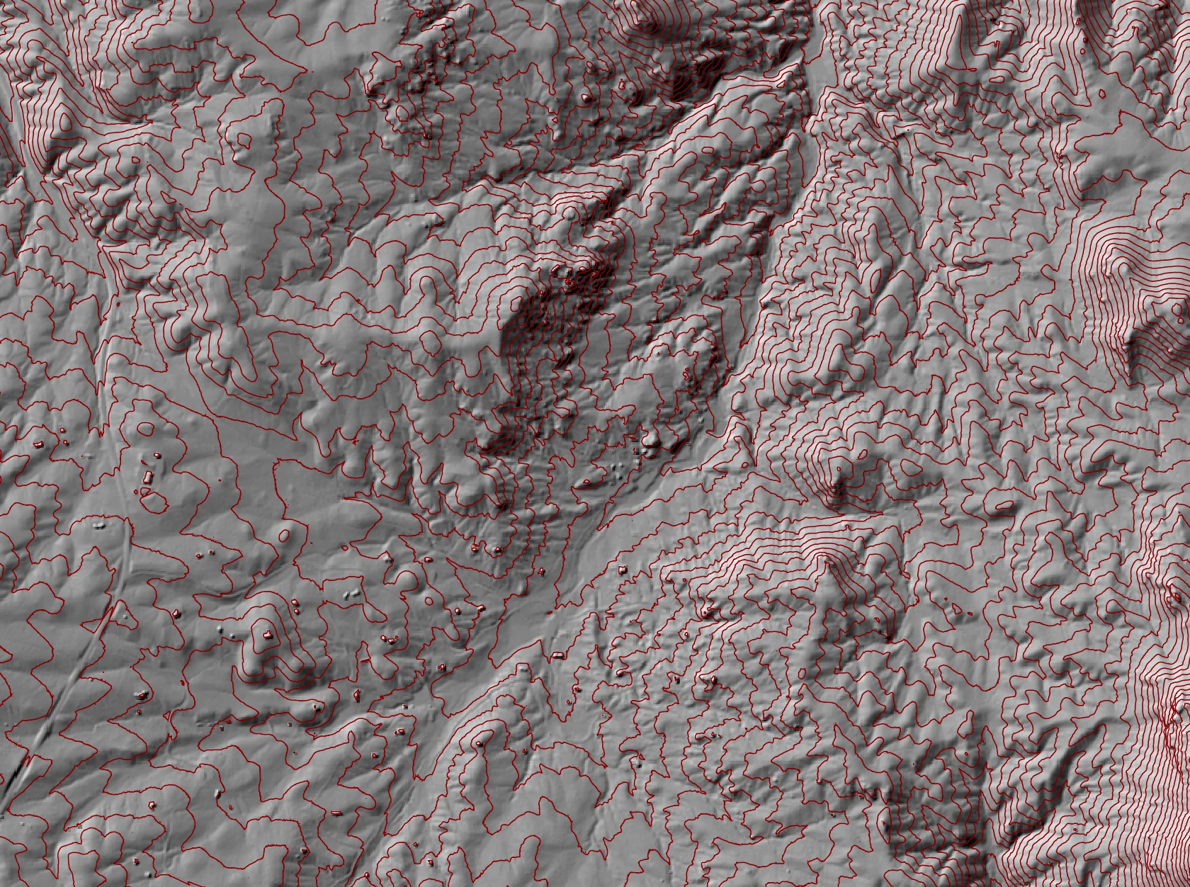
LidarContour
Note this tool is part of a WhiteboxTools extension product. Please visit Whitebox Geospatial Inc. for information about purchasing a license activation key (https://www.whiteboxgeo.com/extension-pricing/).
This tool can be used to create a contour (i.e. isolines
of elevation values) vector coverage from an input LiDAR points data set (--input). The tool works by first
creating a triangulation of the input LiDAR points. The user must specify the
contour interval (--interval), or vertical spacing between contour lines. The --smooth parameter can
be used to increase or decrease the degree to which contours are smoothed. This parameter should be an
odd integer value (0, 1, 3, 5...), with 0 indicating no smoothing. The tool can interpolate
contours based on the LiDAR point elevation values, intensity data, or the user data field (--parameter),
with 'elevation' as the default parameter. LiDAR points may be excluded from the contouring process based
on a number of criteria, including their return value (--returns, which may be 'all', 'last', 'first'),
their class value (--exclude_cls), and whether they fall outside of a user-specified elevation range
(--minz and --maxz). The optional --max_triangle_edge_length parameter can be used to exclude
the output of contours within areas that are sparsely populated areas of the data set, where the triangles
formed by the Delaunay triangulation are too large. This is often the case within bodies of water; long
and narrow triangular facets can also occur within the concave portions of the hull, or polygon enclosing,
the points, when the data have an irregular shaped extent. Setting this parameter can help alleviate the
problem of contouring beyond the data footprint.
Like many of the LiDAR tools, both the --input and --output parameters are optional. If these
parameters are not specified by the user, the tool will search for all LAS files contained within the
current WhiteboxTools working directory. This feature can be useful when you need to contour a large
number of LiDAR tiles. This batch processing mode enables the tool to enable parallel data processing,
which can significantly improve the efficiency of data conversion for datasets with many LiDAR tiles.
When run in this batch mode, the output file (--output) also need not be specified; the tool will
instead create an output file with the same name as each input LiDAR file, but with the .shp extension.
It is important to note that contouring is better suited to well-defined surfaces (e.g. the ground surface or building heights), rather than volume features, such as vegetation, which tend to produce extremely complex contour sets. It is advisable to use this tool with last-returns and/or ground-classified point returns. If the input data set does not contain ground classification, consider pre-processing with the LidarGroundPointFilter tool.
See Also: ContoursFromPoints, ContoursFromRaster, LidarGroundPointFilter
Parameters:
| Flag | Description |
|---|---|
| -i, --input | Name of the input LiDAR points |
| -o, --output | Name of the output vector lines file |
| --interval | Contour interval |
| --base | Base contour |
| --smooth | Smoothing filter size (in num. points), e.g. 3, 5, 7, 9, 11 |
| -p, --parameter | Interpolation parameter; options are 'elevation' (default), 'intensity', 'user_data' |
| --returns | Point return types to include; options are 'all' (default), 'last', 'first' |
| --exclude_cls | Optional exclude classes from interpolation; Valid class values range from 0 to 18, based on LAS specifications. Example, --exclude_cls='3,4,5,6,7,18' |
| --minz | Optional minimum elevation for inclusion in interpolation |
| --maxz | Optional maximum elevation for inclusion in interpolation |
| --max_triangle_edge_length | Optional maximum triangle edge length; triangles larger than this size will not be gridded |
Python function:
wbt.lidar_contour(
    i=None,
    output=None,
    interval=10.0,
    base=0.0,
    smooth=5,
    parameter="elevation",
    returns="all",
    exclude_cls=None,
    minz=None,
    maxz=None,
    max_triangle_edge_length=None,
    callback=default_callback
)
Command-line Interface:
>> ./whitebox_tools -r=LidarContour -i=input.las ^
-o=output.las --interval=5.0 --parameter=elevation ^
--returns=last --smooth=9
Source code is unavailable due to proprietary license.
Author: Whitebox Geospatial Inc. (c)
Created: 21/06/2021
Last Modified: 21/06/2021
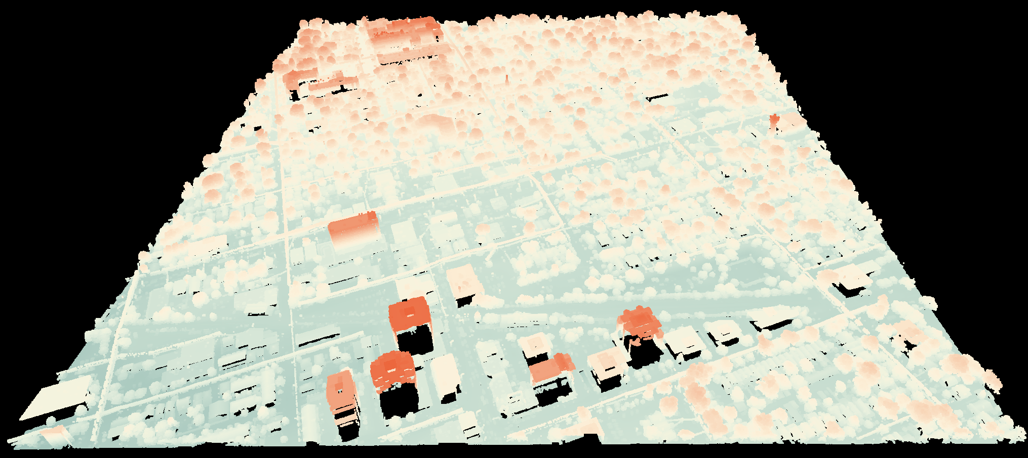
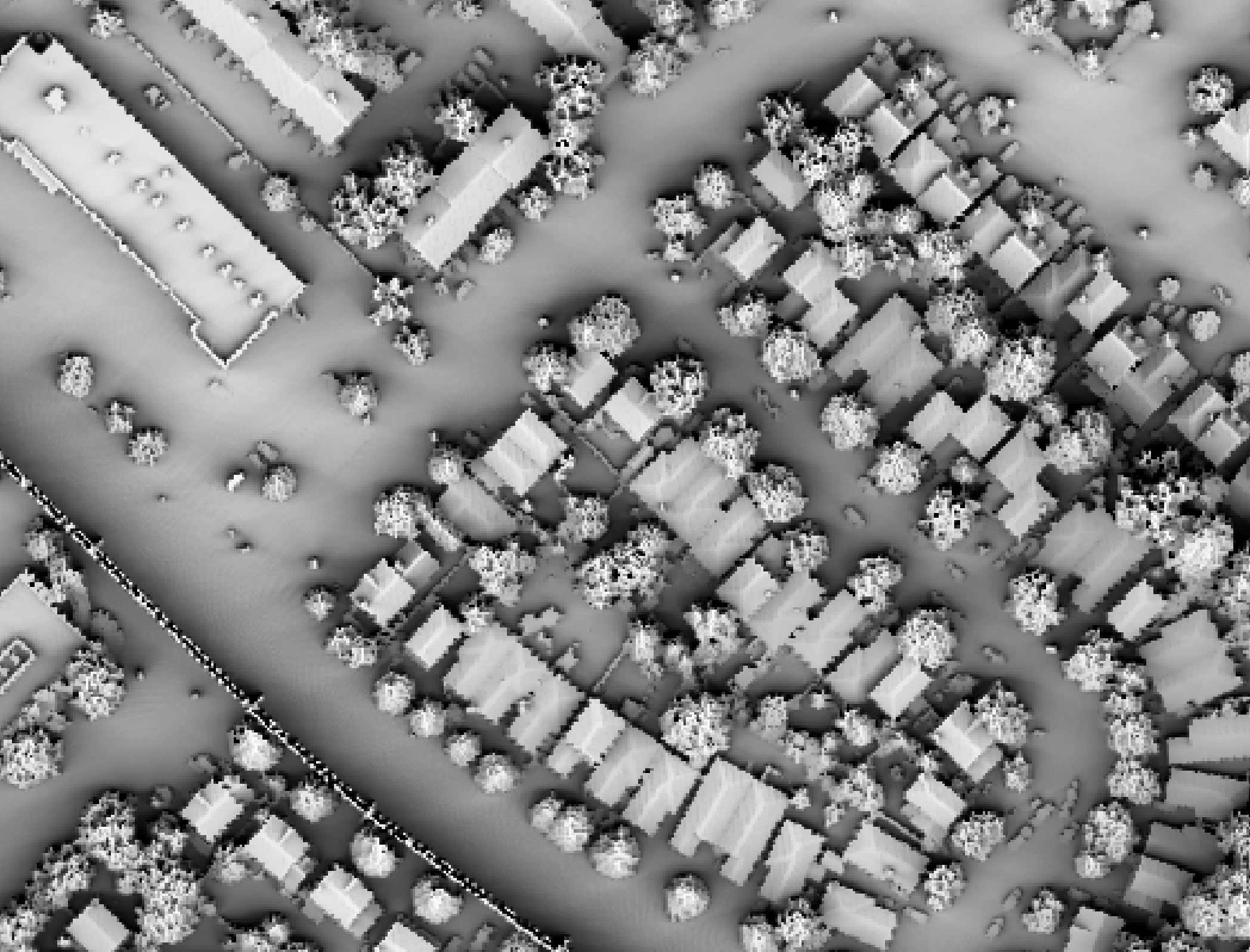
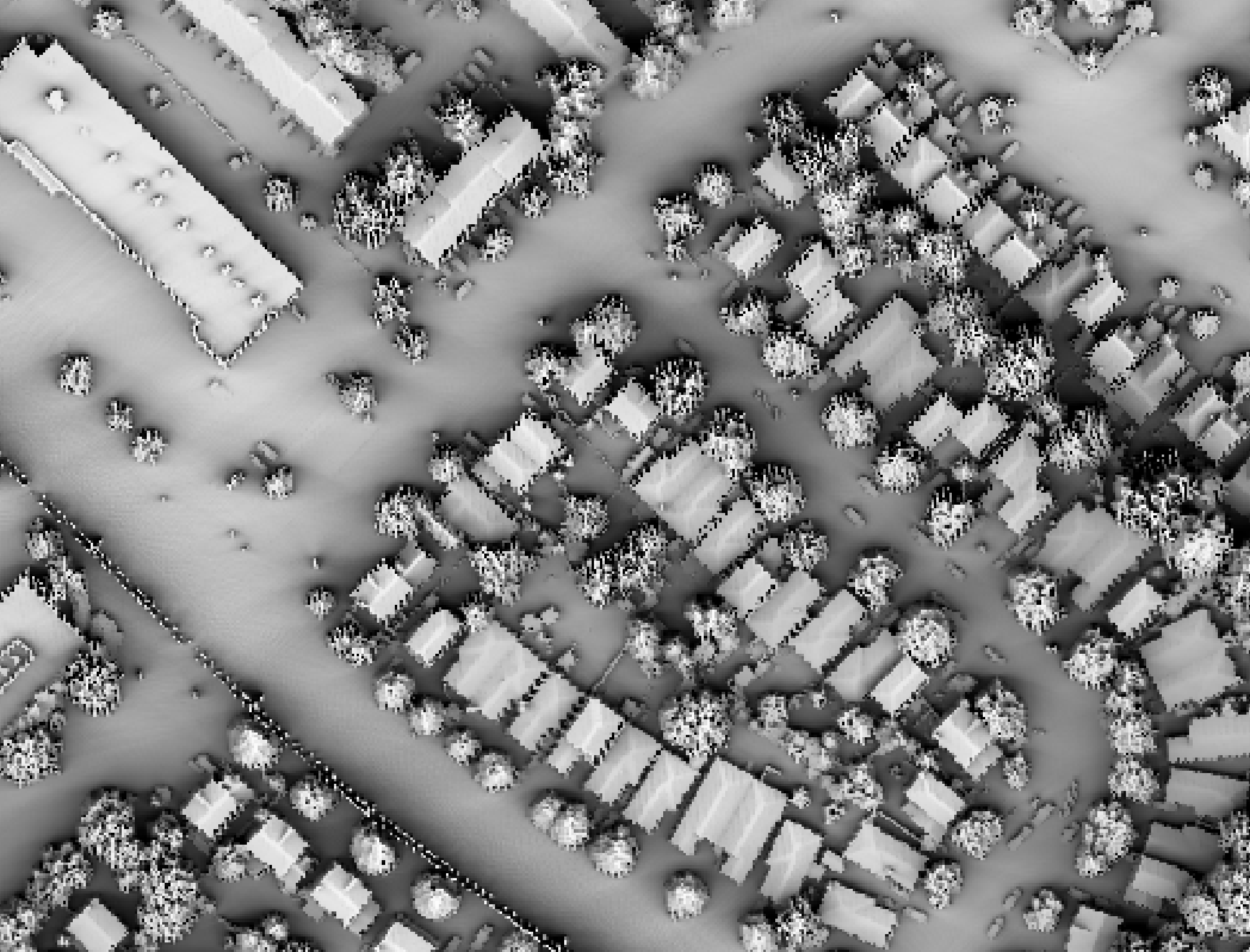
LidarDigitalSurfaceModel
This tool creates a digital surface model (DSM) from a LiDAR point cloud. A DSM reflects the elevation of the tops
of all off-terrain objects (i.e. non-ground features) contained within the data set. For example, a DSM will model
the canopy top as well as building roofs. This is in stark contrast to a bare-earth digital elevation model (DEM),
which models the ground surface without off-terrain objects present. Bare-earth DEMs can be derived from LiDAR data
by interpolating last-return points using one of the other LiDAR interpolators (e.g. LidarTINGridding). The algorithm
used for interpolation in this tool is based on gridding a triangulation (TIN) fit to top-level points in the
input LiDAR point cloud. All points in the input LiDAR data set that are below other neighbouring points, within
a specified search radius (--radius), and that have a large inter-point slope, are filtered out. Thus, this tool
will remove the ground surface beneath as well as any intermediate points within a forest canopy, leaving only the
canopy top surface to be interpolated. Similarly, building wall points and any ground points beneath roof overhangs
will also be remove prior to interpolation. Note that because the ground points beneath overhead wires and utility
lines are filtered out by this operation, these features tend to be appear as 'walls' in the output DSM. If these
points are classified in the input LiDAR file, you may wish to filter them out before using this tool (FilterLidarClasses).
The following images show the differences between creating a DSM using the LidarDigitalSurfaceModel and by interpolating first-return points only using the LidarTINGridding tool respectively. Note, the images show TimeInDaylight, which is a more effective way of hillshading DSMs than the traditional Hillshade method. Compare how the DSM created LidarDigitalSurfaceModel tool (above) has far less variability in areas of tree-cover, more effectively capturing the canopy top. As well, notice how building rooftops are more extensive and straighter in the LidarDigitalSurfaceModel DSM image. This is because this method eliminates ground returns beneath roof overhangs before the triangulation operation.
The user must specify the grid resolution of the output raster (--resolution), and optionally, the name of the
input LiDAR file (--input) and output raster (--output). Note that if an input LiDAR file (--input) is not
specified by the user, the tool will search for all valid LiDAR (*.las, *.laz, *.zlidar) files contained within the current
working directory. This feature can be very useful when you need to interpolate a DSM for a large number of LiDAR
files. Not only does this batch processing mode enable the tool to run in a more optimized parallel manner, but it
will also allow the tool to include a small buffer of points extending into adjacent tiles when interpolating an
individual file. This can significantly reduce edge-effects when the output tiles are later mosaicked together.
When run in this batch mode, the output file (--output) also need not be specified; the tool will instead create
an output file with the same name as each input LiDAR file, but with the .tif extension. This can provide a very
efficient means for processing extremely large LiDAR data sets.
Users may also exclude points from the interpolation if they fall below or above the minimum (--minz) or
maximum (--maxz) thresholds respectively. This can be a useful means of excluding anomalously high or low
points. Note that points that are classified as low points (LAS class 7) or high noise (LAS class 18) are
automatically excluded from the interpolation operation.
Triangulation will generally completely fill the convex hull containing the input point data. This can sometimes
result in very long and narrow triangles at the edges of the data or connecting vertices on either side of void
areas. In LiDAR data, these void areas are often associated with larger waterbodies, and triangulation can result
in very unnatural interpolated patterns within these areas. To avoid this problem, the user may specify a the
maximum allowable triangle edge length (max_triangle_edge_length) and all grid cells within triangular facets
with edges larger than this threshold are simply assigned the NoData values in the output DSM. These NoData areas
can later be better dealt with using the FillMissingData tool after interpolation.
See Also: LidarTINGridding, FilterLidarClasses, FillMissingData, TimeInDaylight
Parameters:
| Flag | Description |
|---|---|
| -i, --input | Input LiDAR file (including extension) |
| -o, --output | Output raster file (including extension) |
| --resolution | Output raster's grid resolution |
| --radius | Search Radius |
| --minz | Optional minimum elevation for inclusion in interpolation |
| --maxz | Optional maximum elevation for inclusion in interpolation |
| --max_triangle_edge_length | Optional maximum triangle edge length; triangles larger than this size will not be gridded |
Python function:
wbt.lidar_digital_surface_model(
    i=None,
    output=None,
    resolution=1.0,
    radius=0.5,
    minz=None,
    maxz=None,
    max_triangle_edge_length=None,
    callback=default_callback
)
Command-line Interface:
>>./whitebox_tools -r=LidarDigitalSurfaceModel -v ^
--wd="/path/to/data/" -i=file.las -o=outfile.tif ^
--returns=last --resolution=2.0 --exclude_cls='3,4,5,6,7,18' ^
--max_triangle_edge_length=5.0
Author: Dr. John Lindsay
Created: 16/08/2020
Last Modified: 16/08/2020
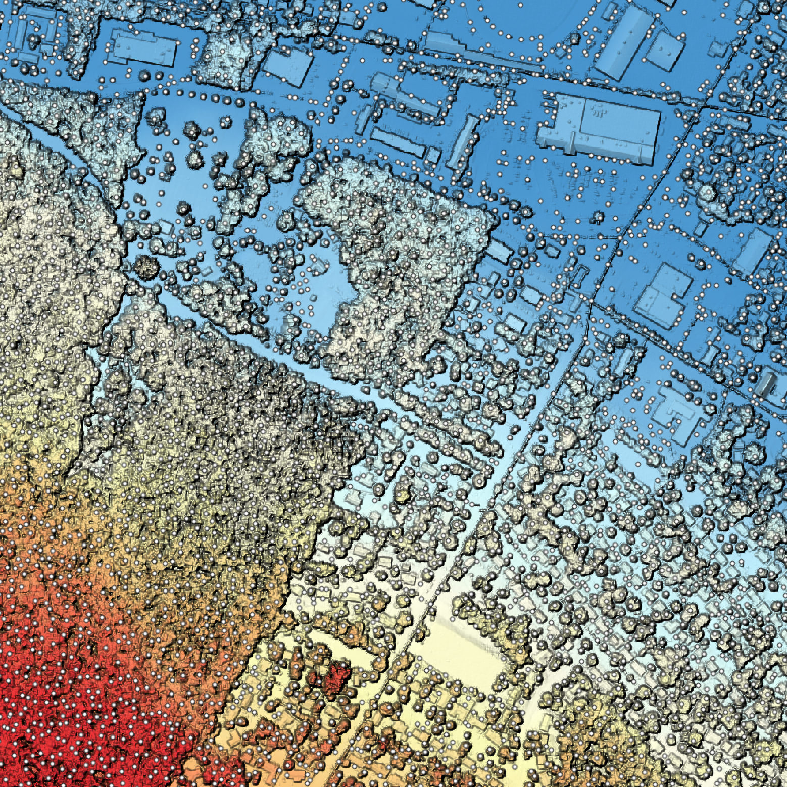
LidarEigenvalueFeatures
Note this tool is part of a WhiteboxTools extension product. Please contact Whitebox Geospatial Inc. for information about purchasing a license activation key (https://www.whiteboxgeo.com/extension-pricing/).
This tool can be used to measure eigenvalue-based features that describe the characteristics of the local
neighbourhood surrounding each point in an input LiDAR file (--input). These features can then be used in
point classification applications, or as the basis for point filtering (FilterLidar) or modifying point
properties (ModifyLidar).
The algorithm begins by using the x, y, z coordinates of the points within a local spherical neighbourhood to calculate a covariance matrix. The three eigenvalues λ1, λ2, λ3 are then derived from the covariance matrix decomposition such that λ1 > λ2 > λ3. The eigenvalues are then used to describe the extent to which the neighbouring points can be characterized by a linear, planar, or volumetric distribution, by calculating the following three features:
linearity = (λ1 - λ2) / λ1
planarity = (λ2 - λ3) / λ1
sphericity = λ3 / λ1
In the case of a neighbourhood containing a 1-dimensional line, the first of the three components will possess most of data variance, with very little contained within λ2 and λ3, and linearity will be nearly equal to 1.0. If the local neighbourhood contains a 2-dimensional plane, the first two components will possess most of the variance, with little variance within λ3, and planarity will be nearly equal to 1.0. Lastly, in the case of a 3-dimensional, random volumetric point distribution, each of the three components will be nearly equal in magnitude and sphericity will be nearly equal to 1.0.
Researchers in the field of LiDAR point classification also frequently define two additional eigenvalue-based features, the omnivariance (low values correspond to planar and linear regions and higher values occur for areas with a volumetric point distribution, such as vegetation), and the eigentropy, which is related to the Shannon entropy and is a measure of the unpredictability of the distribution of points in the neighbourhood:
omnivariance = (λ1 ⋅ λ2 ⋅ λ3)1/3
eigentropy = -e1 ⋅ lne1 - e2 ⋅ lne2 - e3 ⋅ lne3
where e1, e2, and e3 are the normalized eigenvalues.
In addition to the eigenvalues, the eigendecomposition of the symmetric covariance matrix also yields the three eigenvectors, which describe the transformation coefficients of the principal components. The first two eigenvectors represent the basis of the plane resulting from the orthogonal regression analysis, while the third eigenvector represents the plane normal. From this normal, it is possible to calculate the slope of the plane, as well as the orthogonal distance between each point and the neighbourhood fitted plane, i.e. the point residual.
This tool outputs a binary file (*.eigen; --output) that contains a total of 10 features for each
point in the input file, including the point_num (for reference), lambda1, lambda2, lambda3, linearity,
planarity, sphericity, omnivariance, eigentropy, slope, and residual. Users should bear in mind
that most of these features describe the properties of the distribution of points within a spherical neighbourhood
surrounding each point in the input file, rather than a characteristic of the point itself. The only one
of the ten features that is a point property is the residual. Points for which the planarity value is high and the
residual value is low may be assumed to be part of the plane that dominate the structure of their neighbourhoods.
In addition to the binary data *.eigen file, the tool will also output a sidecar file,
with a *.eigen.json extension, which describes the structure of the raw binary data file.
Local neighbourhoods are spherical in shape and the size of each neighbourhood is characterized by the
--num_neighbours and --radius parameters. If the optional --num_neighbours parameter is specified,
the size of the neighbourhood will vary by point, increasing or decreasing to encompass the specified number
of neighbours (notice that this value does not include the point itself). If the optional --radius parameter
is specified in addition to a number of neighbours, the specified radius value will serve as a upper-bound
and neighbouring points that are beyond this radial distance to the centre point will be excluded. If a radius
search distance is specified but the --num_neighbours parameter is not, then a constant search distance will
be used for each point in the input file, resulting in varying number of points within local neighbourhoods,
depending on local point densities. If point density varies significantly in the input file, then use of the
--num_neighbours parameter may be advisable. Notice that at least one of the two parameters must be specified.
In cases where the number of neighbouring points is fewer than eight, each of the output feature values will
be set to 0.0.
Note that if the user does not specify the optional input LiDAR file, the tool will search for all valid LiDAR (*.las, *.laz, *.zlidar) files contained within the current working directory. This feature can be useful for processing a large number of LiDAR files in batch mode.
The binary data file (*.eigen) can be used directly by the FilterLidar and ModifyLidar tools, and will
be automatically read by the tools when the *.eigen and *.eigen.json files are present in the same
folder as the accompanying source LiDAR file. This allows users to apply
data filters, or to modify point properties, using these point neighbourhood features. For example, the
statement, rgb=(int(linearity*255), int(planarity*255), int(sphericity*255)), used with the ModifyLidar
tool, can render the point RGB colour values based on some of the eigenvalue features, allowing users to
visually identify linear features (red), planar features (green), and volumetric regions (blue).
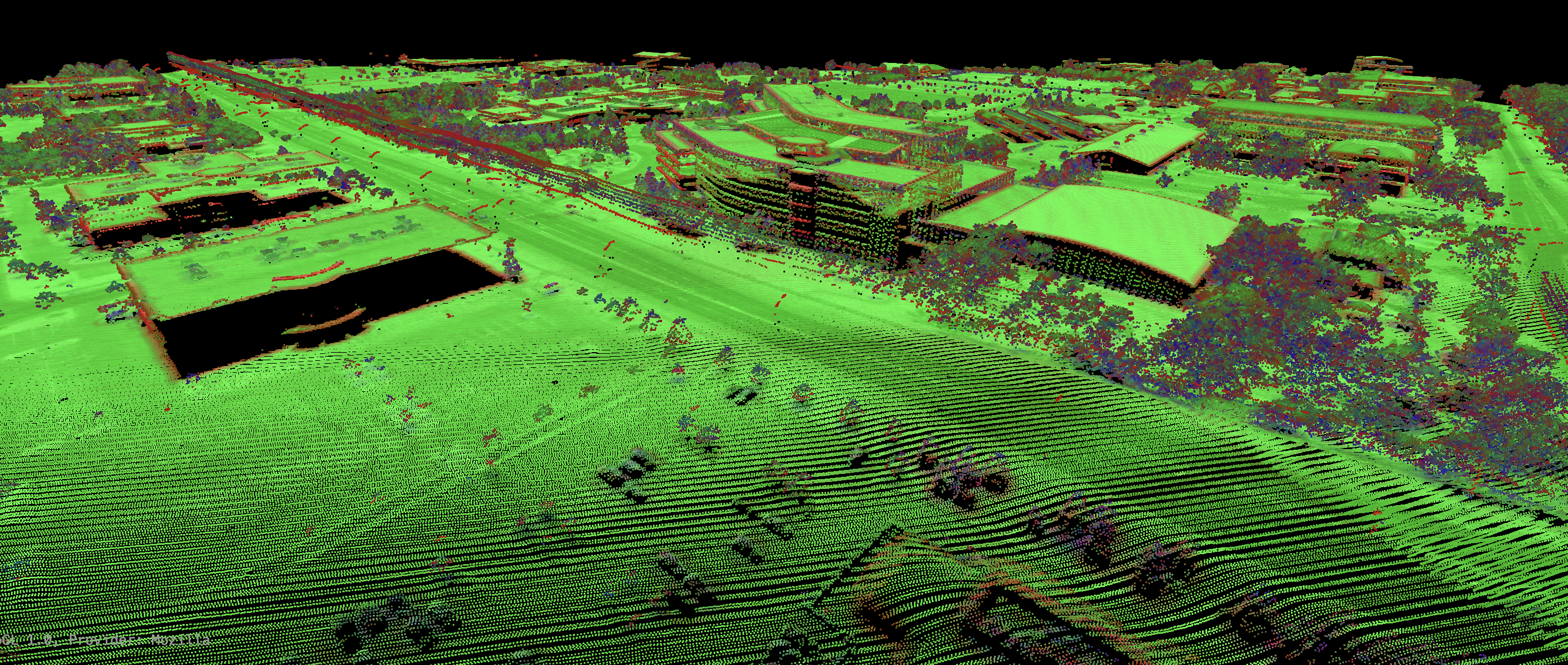
Additionally, these features data can also be readily incorporated into a Python-based point analysis or classification. As an example, the following script reads in a *.eigen binary data file for direct manipulation and analysis:
import numpy as np

dt = np.dtype([
('point_num', '<u8'),
('lambda1', '<f4'),
('lambda2', '<f4'),
('lambda3', '<f4'),
('linearity', '<f4'),
('planarity', '<f4'),
('sphericity', '<f4'),
('omnivariance', '<f4'),
('eigentropy', '<f4'),
('slope', '<f4'),
('resid', '<f4')
])

with open('/Users/johnlindsay/Documents/data/aaa2.eigen', 'rb') as f:
b = f.read()

pt_features = np.frombuffer(b, dt)

# Print the first 100 point features to demonstrate
for i in range(100):
print(f"{pt_features['point_num'][i]} {pt_features['linearity'][i]} {pt_features['planarity'][i]} {pt_features['sphericity'][i]}")


print("Done!")
References:
Chehata, N., Guo, L., & Mallet, C. (2009). Airborne lidar feature selection for urban classification using random forests. In Laser Scanning IAPRS, Vol. XXXVIII, Part 3/W8 – Paris, France, September 1-2, 2009.
Gross, H., Jutzi, B., & Thoennessen, U. (2007). Segmentation of tree regions using data of a full-waveform laser. International Archives of Photogrammetry, Remote Sensing and Spatial Information Sciences, 36(part 3), W49A.
Niemeyer, J., Mallet, C., Rottensteiner, F., & Sörgel, U. (2012). Conditional Random Fields for the Classification of LIDAR Point Clouds. In XXII ISPRS Congress at Melbourne, ISPRS Annals of the Photogrammetry, Remote Sensing and Spatial Information Sciences (Vol. 3).
West, K. F., Webb, B. N., Lersch, J. R., Pothier, S., Triscari, J. M., & Iverson, A. E. (2004). Context-driven automated target detection in 3D data. In Automatic Target Recognition XIV (Vol. 5426, pp. 133-143). SPIE.
See Also: FilterLidar, ModifyLidar, SortLidar, SplitLidar
Parameters:
| Flag | Description |
|---|---|
| -i, --input | Name of the input LiDAR points |
| --num_neighbours | Number of neighbours used in search |
| --radius | Search distance used in neighbourhood search |
Python function:
wbt.lidar_eigenvalue_features(
    i=None,
    num_neighbours=None,
    radius=None,
    callback=default_callback
)
Command-line Interface:
>> ./whitebox_tools -r=LidarEigenvalueFeatures -i=input.las ^
-o=output.las --radius=2.5
Source code is unavailable due to proprietary license.
Author: Whitebox Geospatial Inc. (c)
Created: 18/02/2022
Last Modified: 25/02/2022
LidarElevationSlice
This tool can be used to either extract or classify the elevation values (z) of LiDAR points within
a specified elevation range (slice). In addition to the names of the input and output LiDAR files
(--input and --output), the user must specify the lower (--minz) and upper (--maxz) bounds of
the elevation range. By default, the tool will only output points within the elevation slice, filtering
out all points lying outside of this range. If the --class parameter is used, the tool will operate
by assigning a class value (--inclassval) to the classification bit of points within the slice and
another class value (--outclassval) to those points falling outside the range.
See Also: LidarRemoveOutliers, LidarClassifySubset
Parameters:
| Flag | Description |
|---|---|
| -i, --input | Input LiDAR file |
| -o, --output | Output LiDAR file |
| --minz | Minimum elevation value (optional) |
| --maxz | Maximum elevation value (optional) |
| --class | Optional boolean flag indicating whether points outside the range should be retained in output but reclassified |
| --inclassval | Optional parameter specifying the class value assigned to points within the slice |
| --outclassval | Optional parameter specifying the class value assigned to points within the slice |
Python function:
wbt.lidar_elevation_slice(
    i,
    output,
    minz=None,
    maxz=None,
    cls=False,
    inclassval=2,
    outclassval=1,
    callback=default_callback
)
Command-line Interface:
>>./whitebox_tools -r=LidarElevationSlice -v ^
--wd="/path/to/data/" -i="input.las" -o="output.las" ^
--minz=100.0 --maxz=250.0
>>./whitebox_tools ^
-r=LidarElevationSlice -v -i="/path/to/data/input.las" ^
-o="/path/to/data/output.las" --minz=100.0 --maxz=250.0 ^
--class
>>./whitebox_tools -r=LidarElevationSlice -v ^
-i="/path/to/data/input.las" -o="/path/to/data/output.las" ^
--minz=100.0 --maxz=250.0 --inclassval=1 --outclassval=0
Author: Dr. John Lindsay
Created: 02/06/2017
Last Modified: 18/10/2019
LidarGroundPointFilter
This tool can be used to perform a slope-based classification, or filtering (i.e. removal), of
non-ground points within a LiDAR point-cloud. The user must specify the name of the input and output
LiDAR files (--input and --output). Inter-point slopes are compared between pair of points
contained within local neighbourhoods of size --radius. Neighbourhoods with fewer than the
user-specified minimum number of points (--min_neighbours) are extended until the minimum point
number is equaled or exceeded. Points that are above neighbouring points by the minimum
(--height_threshold) and have an inter-point slope greater than the user-specifed threshold
(--slope_threshold) are considered non-ground points and are either optionally (--classify)
excluded from the output point-cloud or assigned the unclassified (value 1) class value.
Slope-based ground-point classification methods suffer from the challenge of uses a constant
slope threshold under varying terrain slopes. Some researchers have developed schemes for varying
the slope threshold based on underlying terrain slopes. LidarGroundPointFilter instead allow the
user to optionally (--slope_norm) normalize the underlying terrain (i.e. flatten the terrain)
using a white top-hat transform. A constant slope threshold may then be used without contributing
to poorer performance under steep topography. Note, that this option, while useful in rugged
terrain, is computationally intensive. If the point-cloud is of a relatively flat terrain,
this option may be excluded.
While this tool is appropriately applied to LiDAR point-clouds, the RemoveOffTerrainObjects tool can be used to remove off-terrain objects from rasterized LiDAR digital elevation models (DEMs).
Reference:
Vosselman, G. (2000). Slope based filtering of laser altimetry data. International Archives of Photogrammetry and Remote Sensing, 33(B3/2; PART 3), 935-942.
See Also: RemoveOffTerrainObjects
Parameters:
| Flag | Description |
|---|---|
| -i, --input | Input LiDAR file |
| -o, --output | Output LiDAR file |
| --radius | Search Radius |
| --min_neighbours | The minimum number of neighbouring points within search areas. If fewer points than this threshold are identified during the fixed-radius search, a subsequent kNN search is performed to identify the k number of neighbours |
| --slope_threshold | Maximum inter-point slope to be considered an off-terrain point |
| --height_threshold | Inter-point height difference to be considered an off-terrain point |
| --classify | Classify points as ground (2) or off-ground (1) |
| --slope_norm | Perform initial ground slope normalization? |
| --height_above_ground | Transform output to height above average ground elevation? |
Python function:
wbt.lidar_ground_point_filter(
    i,
    output,
    radius=2.0,
    min_neighbours=0,
    slope_threshold=45.0,
    height_threshold=1.0,
    classify=True,
    slope_norm=True,
    height_above_ground=False,
    callback=default_callback
)
Command-line Interface:
>>./whitebox_tools -r=LidarGroundPointFilter -v ^
--wd="/path/to/data/" -i="input.las" -o="output.las" ^
--radius=10.0 --min_neighbours=10 --slope_threshold=30.0 ^
--height_threshold=0.5 --classify --slope_norm
Author: Dr. John Lindsay
Created: 02/06/2017
Last Modified: 18/10/2019
LidarHexBinning
The practice of binning point data to form a type of 2D histogram, density plot, or what is sometimes called a heatmap, is quite useful as an alternative for the cartographic display of of very dense points sets. This is particularly the case when the points experience significant overlap at the displayed scale. The LidarPointDensity tool can be used to perform binning based on a regular grid (raster output). This tool, by comparison, bases the binning on a hexagonal grid.
The tool is similar to the CreateHexagonalVectorGrid tool, however instead will
create an output hexagonal grid in which each hexagonal cell possesses a COUNT
attribute which specifies the number of points from an input points file (LAS file)
that are contained within the hexagonal cell. The tool will also calculate the
minimum and maximum elevations and intensity values and outputs these data to the
attribute table.
In addition to the names of the input points file and the output Shapefile, the user must also specify the desired hexagon width (w), which is the distance between opposing sides of each hexagon. The size (s) each side of the hexagon can then be calculated as, s = w / [2 x cos(PI / 6)]. The area of each hexagon (A) is, A = 3s(w / 2). The user must also specify the orientation of the grid with options of horizontal (pointy side up) and vertical (flat side up).
See Also: VectorHexBinning, LidarPointDensity, CreateHexagonalVectorGrid
Parameters:
| Flag | Description |
|---|---|
| -i, --input | Input base file |
| -o, --output | Output vector polygon file |
| --width | The grid cell width |
| --orientation | Grid Orientation, 'horizontal' or 'vertical' |
Python function:
wbt.lidar_hex_binning(
    i,
    output,
    width,
    orientation="horizontal",
    callback=default_callback
)
Command-line Interface:
>>./whitebox_tools -r=LidarHexBinning -v ^
--wd="/path/to/data/" -i=file.las -o=outfile.shp --width=10.0 ^
--orientation=vertical
Author: Dr. John Lindsay
Created: 16/09/2018
Last Modified: 12/10/2018
LidarHillshade
Calculates a hillshade value for points within a LAS file and stores these data in the RGB field.
Parameters:
| Flag | Description |
|---|---|
| -i, --input | Input LiDAR file |
| -o, --output | Output file |
| --azimuth | Illumination source azimuth in degrees |
| --altitude | Illumination source altitude in degrees |
| --radius | Search Radius |
Python function:
wbt.lidar_hillshade(
    i,
    output,
    azimuth=315.0,
    altitude=30.0,
    radius=1.0,
    callback=default_callback
)
Command-line Interface:
>>./whitebox_tools -r=LidarHillshade -v --wd="/path/to/data/" ^
-i="input.las" -o="output.las" --radius=10.0
>>./whitebox_tools ^
-r=LidarHillshade -v --wd="/path/to/data/" -i="input.las" ^
-o="output.las" --azimuth=180.0 --altitude=20.0 --radius=1.0
Author: Dr. John Lindsay
Created: 14/06/2017
Last Modified: 22/10/2019
LidarHistogram
This tool can be used to plot a histogram of data derived from a LiDAR file. The user must specify the
name of the input LAS file (--input), the name of the output HTML file (--output), the parameter
(--parameter) to be plotted, and the amount (in percent) to clip the upper and lower tails of the f
requency distribution (--clip). The LiDAR parameters that can be plotted using LidarHistogram
include the point elevations, intensity values, scan angles, and class values.
Use the LidarPointStats tool instead to examine the spatial distribution of LiDAR points.
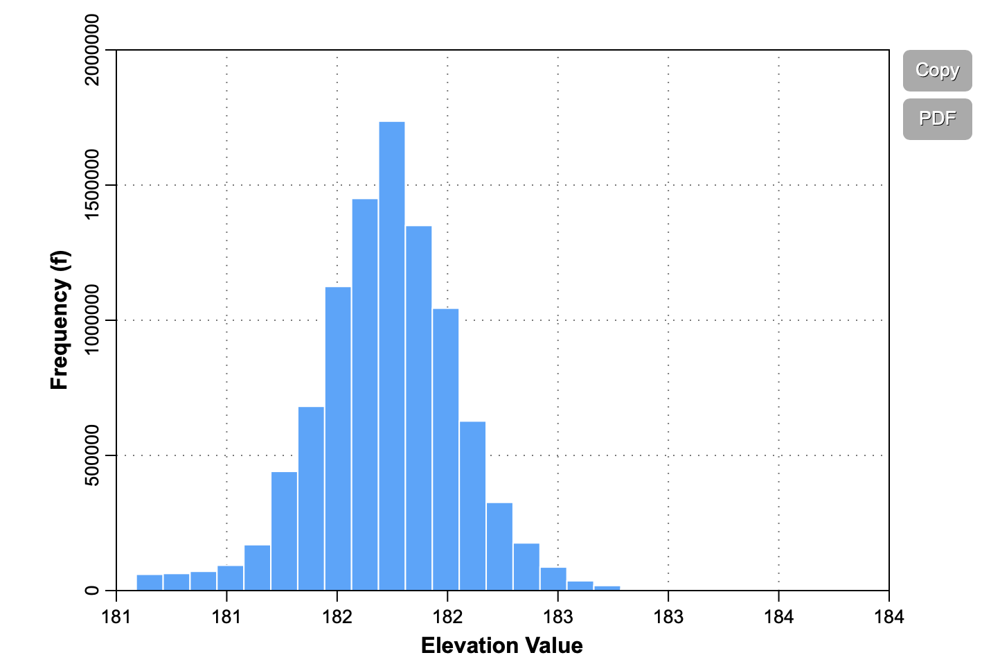
See Also: LidarPointStats
Parameters:
| Flag | Description |
|---|---|
| -i, --input | Input LiDAR file |
| -o, --output | Output HTML file (default name will be based on input file if unspecified) |
| --parameter | Parameter; options are 'elevation' (default), 'intensity', 'scan angle', 'class', 'time' |
| --clip | Amount to clip distribution tails (in percent) |
Python function:
wbt.lidar_histogram(
    i,
    output,
    parameter="elevation",
    clip=1.0,
    callback=default_callback
)
Command-line Interface:
>>./whitebox_tools -r=LidarHistogram -v --wd="/path/to/data/" ^
-i="file1.tif, file2.tif, file3.tif" -o=outfile.htm ^
--contiguity=Bishopsl
Author: Dr. John Lindsay
Created: 23/12/2017
Last Modified: 12/10/2018
LidarIdwInterpolation
This tool interpolates LiDAR files using inverse-distance weighting
(IDW) scheme. The user must specify the value of the IDW weight parameter (--weight). The output grid can be
based on any of the stored LiDAR point parameters (--parameter), including elevation
(in which case the output grid is a digital elevation model, DEM), intensity, class, return number, number of
returns, scan angle, RGB (colour) values, and user data values. Similarly, the user may specify which point
return values (--returns) to include in the interpolation, including all points, last returns (including single
return points), and first returns (including single return points).
The user must specify the grid resolution of the output raster (--resolution), and optionally, the name of the
input LiDAR file (--input) and output raster (--output). Note that if an input LiDAR file (--input) is not
specified by the user, the tool will search for all valid LiDAR (*.las, *.laz, *.zlidar) files contained within the current
working directory. This feature can be very useful when you need to interpolate a DEM for a large number of LiDAR
files. Not only does this batch processing mode enable the tool to run in a more optimized parallel manner, but it
will also allow the tool to include a small buffer of points extending into adjacent tiles when interpolating an
individual file. This can significantly reduce edge-effects when the output tiles are later mosaicked together.
When run in this batch mode, the output file (--output) also need not be specified; the tool will instead create
an output file with the same name as each input LiDAR file, but with the .tif extension. This can provide a very
efficient means for processing extremely large LiDAR data sets.
Users may excluded points from the interpolation based on point classification values, which follow the LAS
classification scheme. Excluded classes are specified using the --exclude_cls parameter. For example,
to exclude all vegetation and building classified points from the interpolation, use --exclude_cls='3,4,5,6'.
Users may also exclude points from the interpolation if they fall below or above the minimum (--minz) or
maximum (--maxz) thresholds respectively. This can be a useful means of excluding anomalously high or low
points. Note that points that are classified as low points (LAS class 7) or high noise (LAS class 18) are
automatically excluded from the interpolation operation.
The tool will search for the nearest input LiDAR point to each grid cell centre, up to a maximum search distance
(--radius). If a grid cell does not have a LiDAR point within this search distance, it will be assigned the
NoData value in the output raster. In LiDAR data, these void areas are often associated with larger waterbodies.
These NoData areas can later be better dealt with using the FillMissingData tool after interpolation.
See Also: LidarTINGridding, LidarNearestNeighbourGridding, LidarSibsonInterpolation
Parameters:
| Flag | Description |
|---|---|
| -i, --input | Input LiDAR file (including extension) |
| -o, --output | Output raster file (including extension) |
| --parameter | Interpolation parameter; options are 'elevation' (default), 'intensity', 'class', 'return_number', 'number_of_returns', 'scan angle', 'rgb', 'user data' |
| --returns | Point return types to include; options are 'all' (default), 'last', 'first' |
| --resolution | Output raster's grid resolution |
| --weight | IDW weight value |
| --radius | Search Radius |
| --exclude_cls | Optional exclude classes from interpolation; Valid class values range from 0 to 18, based on LAS specifications. Example, --exclude_cls='3,4,5,6,7,18' |
| --minz | Optional minimum elevation for inclusion in interpolation |
| --maxz | Optional maximum elevation for inclusion in interpolation |
Python function:
wbt.lidar_idw_interpolation(
    i=None,
    output=None,
    parameter="elevation",
    returns="all",
    resolution=1.0,
    weight=1.0,
    radius=2.5,
    exclude_cls=None,
    minz=None,
    maxz=None,
    callback=default_callback
)
Command-line Interface:
>>./whitebox_tools -r=LidarIdwInterpolation -v ^
--wd="/path/to/data/" -i=file.las -o=outfile.tif ^
--resolution=2.0 --radius=5.0"
./whitebox_tools ^
-r=LidarIdwInterpolation --wd="/path/to/data/" -i=file.las ^
-o=outfile.tif --resolution=5.0 --weight=2.0 --radius=2.0 ^
--exclude_cls='3,4,5,6,7,18'
Author: Dr. John Lindsay
Created: 03/07/2017
Last Modified: 19/05/2020
LidarInfo
This tool can be used to print basic information about the data contained within a LAS file, used to store LiDAR data. The reported information will include including data on the header, point return frequency, and classification data and information about the variable length records (VLRs) and geokeys.
Parameters:
| Flag | Description |
|---|---|
| -i, --input | Input LiDAR file |
| -o, --output | Output HTML file for summary report |
| --density | Flag indicating whether or not to calculate the average point density and nominal point spacing |
| --vlr | Flag indicating whether or not to print the variable length records (VLRs) |
| --geokeys | Flag indicating whether or not to print the geokeys |
Python function:
wbt.lidar_info(
    i,
    output,
    density=True,
    vlr=True,
    geokeys=True,
    callback=default_callback
)
Command-line Interface:
>>./whitebox_tools -r=LidarInfo -v --wd="/path/to/data/" ^
-i=file.las --vlr --geokeys"
./whitebox_tools -r=LidarInfo ^
--wd="/path/to/data/" -i=file.las
Author: Dr. John Lindsay
Created: 01/06/2017
Last Modified: 30/01/2022
LidarJoin
This tool can be used to merge multiple LiDAR LAS files into a single output LAS file. Due to their large size, LiDAR data sets are often tiled into smaller, non-overlapping tiles. Sometimes it is more convenient to combine multiple tiles together for data processing and LidarJoin can be used for this purpose.
See Also: LidarTile
Parameters:
| Flag | Description |
|---|---|
| -i, --inputs | Input LiDAR files |
| -o, --output | Output LiDAR file |
Python function:
wbt.lidar_join(
    inputs,
    output,
    callback=default_callback
)
Command-line Interface:
>>./whitebox_tools -r=LidarJoin -v --wd="/path/to/data/" ^
-i="file1.las, file2.las, file3.las" -o=outfile.las"
Author: Dr. John Lindsay
Created: 21/06/2017
Last Modified: 29/08/2018
LidarKappaIndex
This tool performs a kappa index of agreement (KIA) analysis on the classification values of two LiDAR (LAS) files. The output report HTML file should be displayed automatically but can also be displayed afterwards in any web browser. As a measure of overall classification accuracy, the KIA is more robust than the percent agreement calculation because it takes into account the agreement occurring by random chance. In addition to the KIA, the tool will output the producer's and user's accuracy, the overall accuracy, and the error matrix. The KIA is often used as a means of assessing the accuracy of an image classification analysis; however the LidarKappaIndex tool performs the analysis on a point-to-point basis, comparing the class values of the points in one input LAS file with the corresponding nearest points in the second input LAS file.
The user must also specify the name and resolution of an output raster file, which is used to show the spatial distribution of class accuracy. Each grid cell contains the overall accuracy, i.e. the points correctly classified divided by the total number of points contained within the cell, expressed as a percentage.
Parameters:
| Flag | Description |
|---|---|
| --i1, --input1 | Input LiDAR classification file |
| --i2, --input2 | Input LiDAR reference file |
| -o, --output | Output HTML file |
| --class_accuracy | Output classification accuracy raster file |
| --resolution | Output raster's grid resolution |
Python function:
wbt.lidar_kappa_index(
    input1,
    input2,
    output,
    class_accuracy,
    resolution=1.0,
    callback=default_callback
)
Command-line Interface:
>>./whitebox_tools -r=LidarKappaIndex -v ^
--wd="/path/to/data/" --i1=class.las --i2=reference.las ^
-o=kia.html --class_accuracy=new_file.tif --resolution=0.5
Author: Dr. John Lindsay
Created: 24/09/2017
Last Modified: 04/01/2019
LidarNearestNeighbourGridding
This tool grids LiDAR files using nearest-neighbour (NN) scheme, that is, each grid cell in the output image will be assigned the parameter value of the point nearest the grid cell centre. This method should not be confused for the similarly named natural-neighbour interpolation (a.k.a Sibson's method). Nearest neighbour gridding is generally regarded as a poor way of interpolating surfaces from low-density point sets and results in the creation of a Voronoi diagram. However, this method has several advantages when applied to LiDAR data. NN gridding is one of the fastest methods for generating raster surfaces from large LiDAR data sets. NN gridding is one of the few interpolation methods, along with triangulation, that will preserve vertical breaks-in-slope, such as occur at the edges of building. This characteristic can be important when using some post-processing methods, such as the RemoveOffTerrainObjects tool. Furthermore, because most LiDAR data sets have remarkably high point densities compared with other types of geographic data, this approach does often produce a satisfactory result; this is particularly true when the point density is high enough that there are multiple points in the majority of grid cells.
The output grid can be based on any of the stored LiDAR point parameters (--parameter), including elevation
(in which case the output grid is a digital elevation model, DEM), intensity, class, return number, number of
returns, scan angle, RGB (colour) values, time, and user data values. Similarly, the user may specify which point
return values (--returns) to include in the interpolation, including all points, last returns (including single
return points), and first returns (including single return points).
The user must specify the grid resolution of the output raster (--resolution), and optionally, the name of the
input LiDAR file (--input) and output raster (--output). Note that if an input LiDAR file (--input) is not
specified by the user, the tool will search for all valid LiDAR (*.las, *.laz, *.zlidar) files contained within the current
working directory. This feature can be very useful when you need to interpolate a DEM for a large number of LiDAR
files. Not only does this batch processing mode enable the tool to run in a more optimized parallel manner, but it
will also allow the tool to include a small buffer of points extending into adjacent tiles when interpolating an
individual file. This can significantly reduce edge-effects when the output tiles are later mosaicked together.
When run in this batch mode, the output file (--output) also need not be specified; the tool will instead create
an output file with the same name as each input LiDAR file, but with the .tif extension. This can provide a very
efficient means for processing extremely large LiDAR data sets.
Users may excluded points from the interpolation based on point classification values, which follow the LAS
classification scheme. Excluded classes are specified using the --exclude_cls parameter. For example,
to exclude all vegetation and building classified points from the interpolation, use --exclude_cls='3,4,5,6'.
Users may also exclude points from the interpolation if they fall below or above the minimum (--minz) or
maximum (--maxz) thresholds respectively. This can be a useful means of excluding anomalously high or low
points. Note that points that are classified as low points (LAS class 7) or high noise (LAS class 18) are
automatically excluded from the interpolation operation.
The tool will search for the nearest input LiDAR point to each grid cell centre, up to a maximum search distance
(--radius). If a grid cell does not have a LiDAR point within this search distance, it will be assigned the
NoData value in the output raster. In LiDAR data, these void areas are often associated with larger waterbodies.
These NoData areas can later be better dealt with using the FillMissingData tool after interpolation.
See Also: LidarTINGridding, LidarIdwInterpolation, LidarTINGridding, RemoveOffTerrainObjects, FillMissingData
Parameters:
| Flag | Description |
|---|---|
| -i, --input | Input LiDAR file (including extension) |
| -o, --output | Output raster file (including extension) |
| --parameter | Interpolation parameter; options are 'elevation' (default), 'intensity', 'class', 'return_number', 'number_of_returns', 'scan angle', 'rgb', 'user data', 'time' |
| --returns | Point return types to include; options are 'all' (default), 'last', 'first' |
| --resolution | Output raster's grid resolution |
| --radius | Search Radius |
| --exclude_cls | Optional exclude classes from interpolation; Valid class values range from 0 to 18, based on LAS specifications. Example, --exclude_cls='3,4,5,6,7,18' |
| --minz | Optional minimum elevation for inclusion in interpolation |
| --maxz | Optional maximum elevation for inclusion in interpolation |
Python function:
wbt.lidar_nearest_neighbour_gridding(
    i=None,
    output=None,
    parameter="elevation",
    returns="all",
    resolution=1.0,
    radius=2.5,
    exclude_cls=None,
    minz=None,
    maxz=None,
    callback=default_callback
)
Command-line Interface:
>>./whitebox_tools -r=LidarNearestNeighbourGridding -v ^
--wd="/path/to/data/" -i=file.las -o=outfile.tif ^
--returns=last --resolution=2.0 --radius=5.0"
./whitebox_tools ^
-r=LidarNearestNeighbourGridding --wd="/path/to/data/" ^
-i=file.las -o=outfile.tif --resolution=5.0 --radius=2.0 ^
--exclude_cls='3,4,5,6,7,18'
Author: Dr. John Lindsay
Created: 05/07/2017
Last Modified: 15/06/2021
LidarPointDensity
Calculates the spatial pattern of point density for a LiDAR data set. When the input/output parameters are not specified, the tool grids all LAS files contained within the working directory.
Parameters:
| Flag | Description |
|---|---|
| -i, --input | Input LiDAR file (including extension) |
| -o, --output | Output raster file (including extension) |
| --returns | Point return types to include; options are 'all' (default), 'last', 'first' |
| --resolution | Output raster's grid resolution |
| --radius | Search radius |
| --exclude_cls | Optional exclude classes from interpolation; Valid class values range from 0 to 18, based on LAS specifications. Example, --exclude_cls='3,4,5,6,7,18' |
| --minz | Optional minimum elevation for inclusion in interpolation |
| --maxz | Optional maximum elevation for inclusion in interpolation |
Python function:
wbt.lidar_point_density(
    i=None,
    output=None,
    returns="all",
    resolution=1.0,
    radius=2.5,
    exclude_cls=None,
    minz=None,
    maxz=None,
    callback=default_callback
)
Command-line Interface:
>>./whitebox_tools -r=LidarPointDensity -v ^
--wd="/path/to/data/" -i=file.las -o=outfile.tif ^
--resolution=2.0 --radius=5.0"
./whitebox_tools ^
-r=LidarPointDensity -v --wd="/path/to/data/" -i=file.las ^
-o=outfile.tif --resolution=5.0 --radius=2.0 ^
--exclude_cls='3,4,5,6,7,18' --palette=light_quant.plt
Author: Dr. John Lindsay
Created: 10/07/2017
Last Modified: 19/05/2020
LidarPointReturnAnalysis
Note this tool is part of a WhiteboxTools extension product. Please visit Whitebox Geospatial Inc. for information about purchasing a license activation key (https://www.whiteboxgeo.com/extension-pricing/).
This performs a quality control check on the return values of points in a LiDAR file. In particular, the tool will search for missing point returns, duplicate point returns, and points for which the return number (r) is larger than the encoded number of returns (n), all of which may be indicative of processing or encoding errors in the input file.
The user must specify the name of the input LiDAR file (--input), and may optionally specify an output
LiDAR file (--output). If no output file is specified, only the text report is generated by the tool. If
an output is specified, the tool will create an output LiDAR file for which missing returns are assigned
class 13, duplicate returns are assigned class 14, points that are both, part of a missing series and are
duplicate returns, are classed 15, and all other non-problemmatic points are assigned class 1. Note, those
points designated as missing in the output image are clearly not so much missing as they are part of a
sequence of points that contain missing returns. Missing points are apparent when the first point in a series
does not have r = 1, when the last point does not have r = n, or the series is non-sequential (e.g.
1/3, 3/3, but no 2/3). This condition may occur because returns are split between tiles. However, when
sequences with missing points are not located near the edges of tiles, it is usually an indication that either
point filtering has taken place during pre-processing or that there is been some kind of processing or encoding
error.
Duplicate points are defined as points that share the same time, scanner channel, r, and n. Note that these points may have different x, y, z coordinates. Duplicate points are always an indication of a processing or encoding error. For example, it may indicate that the scanner channel information from a multi-channel LiDAR sensor has not been encoded when creating the file or has been lost.
No point should have r > n. This always indicates some kind of processing or encoding error when it occurs.
The following is a sample output report generated by this tool:
***************************************
* Welcome to LidarPointReturnAnalysis *
***************************************
The Global Encoding for this file indicates that
the point returns are not synthetic.

Missing Returns:
2441636 (16.336 percent) points are missing

| r | n | Missing Pts |
|---|---|-------------|
| 1 | 2 |     1127770 |
| 2 | 2 |         817 |
| 1 | 3 |      823240 |
| 2 | 3 |         569 |
| 3 | 3 |         718 |
| 1 | 4 |      285695 |
| 2 | 4 |      142890 |
| 3 | 4 |         142 |
| 4 | 4 |         213 |
| 1 | 5 |       29772 |
| 2 | 5 |       19848 |
| 3 | 5 |        9928 |
| 4 | 5 |          18 |
| 5 | 5 |          16 |


Duplicate Returns:
4311021 (28.844 percent) points are duplicates

| r | n | Duplicates |
|---|---|------------|
| 1 | 1 |    2707083 |
| 1 | 2 |     332028 |
| 2 | 2 |     663717 |
| 1 | 3 |      70619 |
| 2 | 3 |     211834 |
| 3 | 3 |     282348 |
| 1 | 4 |       2856 |
| 2 | 4 |       8568 |
| 3 | 4 |      14280 |
| 4 | 4 |      17136 |
| 1 | 5 |         23 |
| 2 | 5 |         69 |
| 3 | 5 |        115 |
| 4 | 5 |        161 |
| 5 | 5 |        184 |


Return Greater Than Num. Returns:
0 (0.000 percent) points have r > n

Writing output LAS file...
Complete!
Elapsed Time (including I/O): 1.959s
Parameters:
| Flag | Description |
|---|---|
| -i, --input | Name of the input LiDAR points |
| -o, --output | Name of the output LiDAR points |
Python function:
wbt.lidar_point_return_analysis(
    i,
    output=None,
    callback=default_callback
)
Command-line Interface:
>> ./whitebox_tools -r=LidarPointReturnAnalysis -i=input.las ^
-o=output.las
Source code is unavailable due to proprietary license.
Author: Whitebox Geospatial Inc. (c)
Created: 13/06/2021
Last Modified: 13/06/2021
LidarPointStats
This tool creates several rasters summarizing the distribution of LiDAR points in a LAS data file.
The user must specify the name of an input LAS file (--input) and the output raster grid
resolution (--resolution). Additionally, the user must specify one or more of the possible
output rasters to create using the various available flags, which include:
| Flag | Meaning |
|---|---|
--num_points | Number of points (returns) in each grid cell |
--num_pulses | Number of pulses in each grid cell |
--avg_points_per_pulse | Average number of points per pulse in each grid cells |
--z_range | Elevation range within each grid cell |
--intensity_range | Intensity range within each grid cell |
--predom_class | Predominant class value within each grid cell |
If no output raster flags are specified, all of the output rasters will be created. All output rasters will have the same base name as the input LAS file but will have a suffix that reflects the statistic type (e.g. _num_pnts, _num_pulses, _avg_points_per_pulse, etc.). Output files will be in the GeoTIFF (*.tif) file format.
When the input/output parameters are not specified, the tool works on all LAS files contained within the working directory.
Notes:
- The num_pulses output is actually the number of pulses with at least one return; specifically it is the sum of the early returns (first and only) in a grid cell. In areas of low reflectance, such as over water surfaces, the system may have emitted a significantly higher pulse rate but far fewer returns are observed.
- The memory requirement of this tool is high, particulalry if the grid resolution is fine and the spatial extent is large.
See Also: LidarBlockMinimum, LidarBlockMaximum
Parameters:
| Flag | Description |
|---|---|
| -i, --input | Input LiDAR file |
| --resolution | Output raster's grid resolution |
| --num_points | Flag indicating whether or not to output the number of points (returns) raster |
| --num_pulses | Flag indicating whether or not to output the number of pulses raster |
| --avg_points_per_pulse | Flag indicating whether or not to output the average number of points (returns) per pulse raster |
| --z_range | Flag indicating whether or not to output the elevation range raster |
| --intensity_range | Flag indicating whether or not to output the intensity range raster |
| --predom_class | Flag indicating whether or not to output the predominant classification raster |
Python function:
wbt.lidar_point_stats(
    i=None,
    resolution=1.0,
    num_points=True,
    num_pulses=False,
    avg_points_per_pulse=True,
    z_range=False,
    intensity_range=False,
    predom_class=False,
    callback=default_callback
)
Command-line Interface:
>>./whitebox_tools -r=LidarPointStats -v ^
--wd="/path/to/data/" -i=file.las --resolution=1.0 ^
--num_points
Author: Dr. John Lindsay
Created: 18/02/2018
Last Modified: 20/05/2020
LidarRansacPlanes
This tool uses the random sample consensus (RANSAC)
method to identify points within a LiDAR point cloud that belong to planar surfaces. RANSAC is a common
method used in the field of computer vision to identify a subset of inlier points in a noisy data set
containing abundant outlier points. Because LiDAR point clouds often contain vegetation points that do not
form planar surfaces, this tool can be used to largely strip vegetation points from the point cloud, leaving
behind the ground returns, buildings, and other points belonging to planar surfaces. If the --classify flag
is used, non-planar points will not be removed but rather will be assigned a different class (1) than the
planar points (0).
The algorithm selects a random sample, of a specified size (--num_samples) of the points from within the
neighbourhood (--radius) surrounding each LiDAR point. The sample is then used to parameterize a planar
best-fit model. The distance between each neighbouring point and the plane is then evaluated; inliers are
those neighbouring points within a user-specified distance threshold (--threshold). Models with at least
a minimum number of inlier points (--model_size) are then accepted. This process of selecting models is
iterated a number of user-specified times (--num_iter).
One of the challenges with identifying planar surfaces in LiDAR point clouds is that these data are usually
collected along scan lines. Therefore, each scan line can potentially yield a vertical planar surface, which
is one reason that some vegetation points remain after applying the RANSAC plane-fitting method. To cope
with this problem, the tool allows the user to specify a maximum planar slope (--max_slope) parameter.
Planes that have slopes greater than this threshold are rejected by the algorithm. This has the side-effect
of removing building walls however.
References:
Fischler MA and Bolles RC. 1981. Random sample consensus: a paradigm for model fitting with applications to image analysis and automated cartography. Commun. ACM, 24(6):381–395.
See Also: LidarSegmentation, LidarGroundPointFilter
Parameters:
| Flag | Description |
|---|---|
| -i, --input | Input LiDAR file |
| -o, --output | Output LiDAR file |
| --radius | Search Radius |
| --num_iter | Number of iterations |
| --num_samples | Number of sample points on which to build the model |
| --threshold | Threshold used to determine inlier points |
| --model_size | Acceptable model size |
| --max_slope | Maximum planar slope |
| --classify | Classify points as ground (2) or off-ground (1) |
| --last_returns | Only include last- and only-return points |
Python function:
wbt.lidar_ransac_planes(
    i,
    output,
    radius=2.0,
    num_iter=50,
    num_samples=5,
    threshold=0.35,
    model_size=8,
    max_slope=80.0,
    classify=False,
    last_returns=False,
    callback=default_callback
)
Command-line Interface:
>>./whitebox_tools -r=LidarRansacPlanes -v ^
--wd="/path/to/data/" -i="input.las" -o="output.las" ^
--radius=10.0 --num_iter=10 --num_samples=5 --threshold=0.25 ^
--max_slope=70.0 --last_returns
Author: Dr. John Lindsay
Created: 23/07/2019
Last Modified: 29/12/2019
LidarRbfInterpolation
Interpolates LAS files using a radial basis function (RBF) scheme. When the input/output parameters are not specified, the tool interpolates all LAS files contained within the working directory.
Parameters:
| Flag | Description |
|---|---|
| -i, --input | Input LiDAR file (including extension) |
| -o, --output | Output raster file (including extension) |
| --parameter | Interpolation parameter; options are 'elevation' (default), 'intensity', 'class', 'return_number', 'number_of_returns', 'scan angle', 'rgb', 'user data' |
| --returns | Point return types to include; options are 'all' (default), 'last', 'first' |
| --resolution | Output raster's grid resolution |
| --num_points | Number of points |
| --exclude_cls | Optional exclude classes from interpolation; Valid class values range from 0 to 18, based on LAS specifications. Example, --exclude_cls='3,4,5,6,7,18' |
| --minz | Optional minimum elevation for inclusion in interpolation |
| --maxz | Optional maximum elevation for inclusion in interpolation |
| --func_type | Radial basis function type; options are 'ThinPlateSpline' (default), 'PolyHarmonic', 'Gaussian', 'MultiQuadric', 'InverseMultiQuadric' |
| --poly_order | Polynomial order; options are 'none' (default), 'constant', 'affine' |
| --weight | Weight parameter used in basis function |
Python function:
wbt.lidar_rbf_interpolation(
    i=None,
    output=None,
    parameter="elevation",
    returns="all",
    resolution=1.0,
    num_points=20,
    exclude_cls=None,
    minz=None,
    maxz=None,
    func_type="ThinPlateSpline",
    poly_order="none",
    weight=5,
    callback=default_callback
)
Command-line Interface:
>>./whitebox_tools -r=LidarRbfInterpolation -v ^
--wd="/path/to/data/" -i=file.las -o=outfile.tif ^
--resolution=2.0 --radius=5.0
Author: Dr. John Lindsay
Created: 08/11/2019
Last Modified: 19/05/2020
LidarRemoveDuplicates
This tool removes duplicate points from a LiDAR data set. Duplicates are determined
by their x, y, and optionally (--include_z) z coordinates.
See Also: EliminateCoincidentPoints
Parameters:
| Flag | Description |
|---|---|
| -i, --input | Input LiDAR file |
| -o, --output | Output LiDAR file |
| --include_z | Include z-values in point comparison? |
Python function:
wbt.lidar_remove_duplicates(
    i,
    output,
    include_z=False,
    callback=default_callback
)
Command-line Interface:
>>./whitebox_tools -r=LidarRemoveDuplicates -v ^
--wd="/path/to/data/" -i="input.las" -o="output.las"
Author: Dr. John Lindsay
Created: 01/03/2018
Last Modified: 18/10/2019
LidarRemoveOutliers
This tool will filter out points from a LiDAR point cloud if the absolute elevation difference between a point and the averge elevation of its neighbourhood, calculated without the point, exceeds a threshold (elev_diff).
Parameters:
| Flag | Description |
|---|---|
| -i, --input | Input LiDAR file |
| -o, --output | Output LiDAR file |
| --radius | Search Radius |
| --elev_diff | Max. elevation difference |
| --use_median | Optional flag indicating whether to use the difference from median elevation rather than mean |
| --classify | Classify points as ground (2) or off-ground (1) |
Python function:
wbt.lidar_remove_outliers(
    i,
    output,
    radius=2.0,
    elev_diff=50.0,
    use_median=False,
    classify=True,
    callback=default_callback
)
Command-line Interface:
>>./whitebox_tools -r=LidarRemoveOutliers -v ^
--wd="/path/to/data/" -i="input.las" -o="output.las" ^
--radius=10.0 --elev_diff=25.0 --use_median
Author: Dr. John Lindsay
Created: 06/02/2018
Last Modified: 18/10/2019
LidarRooftopAnalysis
This tool can be used to identify roof segments in a LiDAR point cloud.
See Also: ClassifyBuildingsInLidar, ClipLidarToPolygon
Parameters:
| Flag | Description |
|---|---|
| -i, --input | Input LiDAR file |
| --buildings | Input vector build footprint polygons file |
| -o, --output | Output vector polygon file |
| --radius | Search Radius |
| --num_iter | Number of iterations |
| --num_samples | Number of sample points on which to build the model |
| --threshold | Threshold used to determine inlier points (in elevation units) |
| --model_size | Acceptable model size, in points |
| --max_slope | Maximum planar slope, in degrees |
| --norm_diff | Maximum difference in normal vectors, in degrees |
| --azimuth | Illumination source azimuth, in degrees |
| --altitude | Illumination source altitude in degrees |
Python function:
wbt.lidar_rooftop_analysis(
    buildings,
    output,
    i=None,
    radius=2.0,
    num_iter=50,
    num_samples=10,
    threshold=0.15,
    model_size=15,
    max_slope=65.0,
    norm_diff=10.0,
    azimuth=180.0,
    altitude=30.0,
    callback=default_callback
)
Command-line Interface:
>>./whitebox_tools -r=LidarRooftopAnalysis -v ^
--wd="/path/to/data/" -i='data.las' --polygons='buildings.shp' ^
-o='rooftops.shp' --radius=10.0 --num_iter=10 --num_samples=5 ^
--threshold=0.25 --max_slope=70.0
Author: Dr. John Lindsay
Created: 10/06/2020
Last Modified: 10/06/2020
LidarSegmentation
This tool can be used to segment a LiDAR point cloud based on differences in the orientation of fitted planar
surfaces and point proximity. The algorithm begins by attempting to fit planar surfaces to all of the points within
a user-specified radius (--radius) of each point in the LiDAR data set. The planar equation is stored for each
point for which a suitable planar model can be fit. A region-growing algorithm is then used to assign nearby points
with similar planar models. Similarity is based on a maximum allowable angular difference (in degrees) between the
two neighbouring points' plane normal vectors (--norm_diff). The --norm_diff parameter can therefore be thought
of as a way of specifying the magnitude of edges mapped by the region-growing algorithm. By setting this value
appropriately, it is possible to segment each facet of a building's roof. Segment edges for planar points may also
be determined by a maximum allowable height difference (--maxzdiff) between neighbouring points on the same plane.
Points for which no suitable planar model can be fit are assigned to 'volume' (non-planar) segments (e.g. vegetation
points) using a region-growing method that connects neighbouring points based solely on proximity (i.e. all volume
points within radius distance are considered to belong to the same segment).
The resulting point cloud will have both planar segments (largely ground surfaces and building roofs and walls) and volume segments (largely vegetation). Each segment is assigned a random red-green-blue (RGB) colour in the output LAS file. The largest segment in any airborne LiDAR dataset will usually belong to the ground surface. This largest segment will always be assigned a dark-green RGB of (25, 120, 0) by the tool.
This tool uses the random sample consensus (RANSAC)
method to identify points within a LiDAR point cloud that belong to planar surfaces. RANSAC is a common
method used in the field of computer vision to identify a subset of inlier points in a noisy data set
containing abundant outlier points. Because LiDAR point clouds often contain vegetation points that do not
form planar surfaces, this tool can be used to largely strip vegetation points from the point cloud, leaving
behind the ground returns, buildings, and other points belonging to planar surfaces. If the --classify flag
is used, non-planar points will not be removed but rather will be assigned a different class (1) than the
planar points (0).
The algorithm selects a random sample, of a specified size (--num_samples) of the points from within the
neighbourhood (--radius) surrounding each LiDAR point. The sample is then used to parameterize a planar
best-fit model. The distance between each neighbouring point and the plane is then evaluated; inliers are
those neighbouring points within a user-specified distance threshold (--threshold). Models with at least
a minimum number of inlier points (--model_size) are then accepted. This process of selecting models is
iterated a number of user-specified times (--num_iter).
One of the challenges with identifying planar surfaces in LiDAR point clouds is that these data are usually
collected along scan lines. Therefore, each scan line can potentially yield a vertical planar surface, which
is one reason that some vegetation points may be assigned to planes during the RANSAC plane-fitting method. To cope
with this problem, the tool allows the user to specify a maximum planar slope (--max_slope) parameter.
Planes that have slopes greater than this threshold are rejected by the algorithm. This has the side-effect
of removing building walls however.
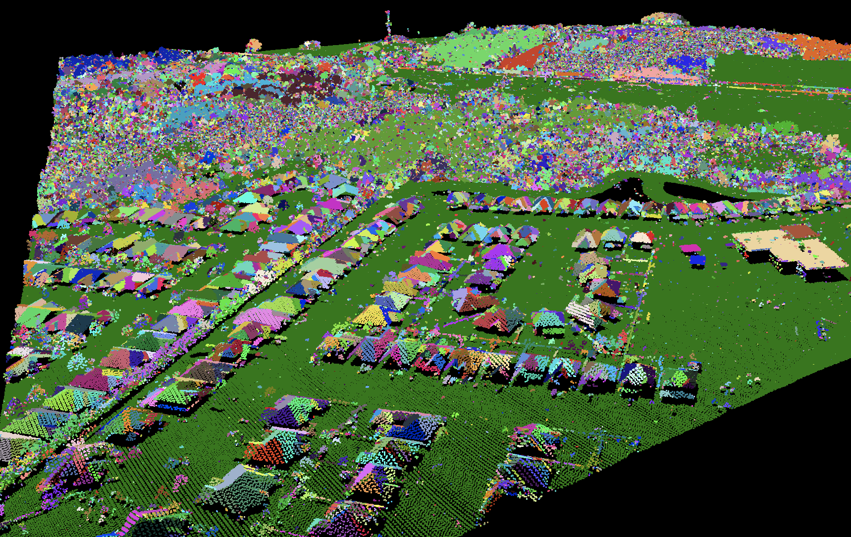
References:
Fischler MA and Bolles RC. 1981. Random sample consensus: a paradigm for model fitting with applications to image analysis and automated cartography. Commun. ACM, 24(6):381–395.
See Also: LidarRansacPlanes, LidarGroundPointFilter
Parameters:
| Flag | Description |
|---|---|
| -i, --input | Input LiDAR file |
| -o, --output | Output LiDAR file |
| --radius | Search Radius |
| --num_iter | Number of iterations |
| --num_samples | Number of sample points on which to build the model |
| --threshold | Threshold used to determine inlier points |
| --model_size | Acceptable model size |
| --max_slope | Maximum planar slope |
| --norm_diff | Maximum difference in normal vectors, in degrees |
| --maxzdiff | Maximum difference in elevation (z units) between neighbouring points of the same segment |
| --classes | Segments don't cross class boundaries |
| --ground | Classify the largest segment as ground points? |
Python function:
wbt.lidar_segmentation(
    i,
    output,
    radius=2.0,
    num_iter=50,
    num_samples=10,
    threshold=0.15,
    model_size=15,
    max_slope=80.0,
    norm_diff=10.0,
    maxzdiff=1.0,
    classes=False,
    ground=False,
    callback=default_callback
)
Command-line Interface:
>>./whitebox_tools -r=LidarSegmentation -v ^
--wd="/path/to/data/" -i="input.las" -o="output.las" ^
--radius=10.0 --num_iter=10 --num_samples=5 --threshold=0.25 ^
--max_slope=70.0
Author: Dr. John Lindsay
Created: 05/12/2017
Last Modified: 12/01/2020
LidarSegmentationBasedFilter
Identifies ground points within LiDAR point clouds using a segmentation based approach.
Parameters:
| Flag | Description |
|---|---|
| -i, --input | Input LiDAR file |
| -o, --output | Output file |
| --dist, --radius | Search Radius |
| --norm_diff | Maximum difference in normal vectors, in degrees |
| --maxzdiff | Maximum difference in elevation (z units) between neighbouring points of the same segment |
| --classify | Classify points as ground (2) or off-ground (1) |
Python function:
wbt.lidar_segmentation_based_filter(
    i,
    output,
    radius=5.0,
    norm_diff=2.0,
    maxzdiff=1.0,
    classify=False,
    callback=default_callback
)
Command-line Interface:
>>./whitebox_tools -r=LidarSegmentationBasedFilter -v ^
--wd="/path/to/data/" -i="input.las" -o="output.las" ^
--radius=10.0 --norm_diff=2.5 --maxzdiff=0.75 --classify
Author: Dr. John Lindsay
Created: 05/12/2017, 2017
Last Modified: 22/10/2019
LidarShift
This tool can be used to shift the x,y,z coordinates of points within a LiDAR file. The user must specify
the name of the input file (--input) and the output file (--output). Additionally, the user must specify
the x,y,z shift values (x_shift, y_shift, z_shift). At least one non-zero shift value is needed
to run the tool. Notice that shifting the x,y,z coordinates of LiDAR points is also possible using the
ModifyLidar tool, which can also be used for more sophisticated point property manipulation (e.g. rotations).
See Also: ModifyLidar, LidarElevationSlice, HeightAboveGround
Parameters:
| Flag | Description |
|---|---|
| -i, --input | Name of the input LiDAR points |
| -o, --output | Name of the output LiDAR points |
| -x, --x_shift | x-shift value, blank for none |
| -y, --y_shift | y-shift value, blank for none |
| -z, --z_shift | z-shift value, blank for none |
Python function:
wbt.lidar_shift(
    i,
    output,
    x_shift="",
    y_shift="",
    z_shift="",
    callback=default_callback
)
Command-line Interface:
>> ./whitebox_tools -r=LidarShift -i=input.las -o=output.las
Source code is unavailable due to proprietary license.
Author: Dr. John Lindsay
Created: 19/01/2022
Last Modified: 19/01/2022
LidarSibsonInterpolation
Note this tool is part of a WhiteboxTools extension product. Please visit Whitebox Geospatial Inc. for information about purchasing a license activation key (https://www.whiteboxgeo.com/extension-pricing/).
This tool interpolates LiDAR files using Sibson's interpolation method, sometimes referred to as natural-neighbour interpolation (not to be confused with nearest-neighbour interpolation, LidarNearestNeighbourGridding). Sibon's method is based on assigning weight to points for which inserting a grid point would result in captured areas of the Voronoi tessellation of the input point set. The larger the captured area, the higher the weight assigned to the associated point. One of the main advantages of this natural neighbour approach to interpolation over similar techniques, such as inverse-distance weighting (IDW LidarIdwInterpolation), is that there is no need to specify a search distance or other interpolation weighting parameters. Sibson's approach frequently provides a very suitable interpolation for LiDAR data. The method requires the calculation of a Delaunay triangulation, from which the Voronoi tessellation is calculated.
The user must specify the value of the IDW weight parameter (--weight). The output grid can be based on any of the
stored LiDAR point parameters (--parameter), including elevation (in which case the output grid is a digital
elevation model, DEM), intensity, class, return number, number of returns, scan angle values, and user data
values. Similarly, the user may specify which point return values (--returns) to include in the interpolation,
including all points, last returns (including single return points), and first returns (including single return
points).
The user must specify the grid resolution of the output raster (--resolution), and optionally, the name of the
input LiDAR file (--input) and output raster (--output). Note that if an input LiDAR file (--input) is not
specified by the user, the tool will search for all valid LiDAR (*.las, *.laz, *.zlidar) files contained within the current
working directory. This feature can be useful when you need to interpolate a DEM for a large number of LiDAR
files. This batch processing mode enables the tool to include a small buffer of points extending into adjacent
tiles when interpolating an individual file. This can significantly reduce edge-effects when the output tiles are
later mosaicked together. When run in this batch mode, the output file (--output) also need not be specified;
the tool will instead create an output file with the same name as each input LiDAR file, but with the .tif
extension. This can provide a very efficient means for processing extremely large LiDAR data sets.
Users may excluded points from the interpolation based on point classification values, which follow the LAS
classification scheme. Excluded classes are specified using the --exclude_cls parameter. For example,
to exclude all vegetation and building classified points from the interpolation, use --exclude_cls='3,4,5,6'.
Users may also exclude points from the interpolation if they fall below or above the minimum (--minz) or
maximum (--maxz) thresholds respectively. This can be a useful means of excluding anomalously high or low
points. Note that points that are classified as low points (LAS class 7) or high noise (LAS class 18) are
automatically excluded from the interpolation operation.
See Also: LidarTINGridding, LidarNearestNeighbourGridding, LidarIdwInterpolation
Parameters:
| Flag | Description |
|---|---|
| -i, --input | Name of the input LiDAR points (leave blank to use all files in WorkingDirectory |
| -o, --output | Output raster file (including extension) |
| -p, --parameter | Interpolation parameter; options are 'elevation' (default), 'intensity', 'class', 'return_number', 'number_of_returns', 'scan angle', 'user_data' |
| --returns | Point return types to include; options are 'all' (default), 'last', 'first' |
| --resolution | Output raster's grid resolution |
| --exclude_cls | Optional exclude classes from interpolation; Valid class values range from 0 to 18, based on LAS specifications. Example, --exclude_cls='3,4,5,6,7,18' |
| --minz | Optional minimum elevation for inclusion in interpolation |
| --maxz | Optional maximum elevation for inclusion in interpolation |
Python function:
wbt.lidar_sibson_interpolation(
    i=None,
    output=None,
    parameter="elevation",
    returns="all",
    resolution=1.0,
    exclude_cls=None,
    minz=None,
    maxz=None,
    callback=default_callback
)
Command-line Interface:
>> ./whitebox_tools -r=LidarSibsonInterpolation -i=file.las ^
-o=outfile.tif -p='elevation' --returns='last' ^
--resolution=1.0 --exclude_cls='3,4,5,6,7,18'
Source code is unavailable due to proprietary license.
Author: Whitebox Geospatial Inc. (c)
Created: 12/04/2021
Last Modified: 12/04/2021
LidarThin
Thins a LiDAR point cloud, reducing point density.
Parameters:
| Flag | Description |
|---|---|
| -i, --input | Input LiDAR file |
| -o, --output | Output LiDAR file |
| --resolution | The size of the square area used to evaluate nearby points in the LiDAR data |
| --method | Point selection method; options are 'first', 'last', 'lowest' (default), 'highest', 'nearest' |
| --save_filtered | Save filtered points to separate file? |
Python function:
wbt.lidar_thin(
    i,
    output,
    resolution=2.0,
    method="lowest",
    save_filtered=False,
    callback=default_callback
)
Command-line Interface:
>>./whitebox_tools -r=LidarThin -v --wd="/path/to/data/" ^
-i=file.las -o=outfile.las --resolution=2.0, --method=first ^
--save_filtered
Author: Dr. John Lindsay
Created: 06/05/2018
Last Modified: 18/10/2019
LidarThinHighDensity
Thins points from high density areas within a LiDAR point cloud.
Parameters:
| Flag | Description |
|---|---|
| -i, --input | Input LiDAR file |
| -o, --output | Output LiDAR file |
| --resolution | Output raster's grid resolution |
| --density | Max. point density (points / m^3) |
| --save_filtered | Save filtered points to separate file? |
Python function:
wbt.lidar_thin_high_density(
    i,
    output,
    density,
    resolution=1.0,
    save_filtered=False,
    callback=default_callback
)
Command-line Interface:
>>./whitebox_tools -r=LidarThinHighDensity -v ^
--wd="/path/to/data/" -i="input.las" -o="output.las" ^
--resolution=1.0 --density=100.0 --save_filtered
Author: Dr. John Lindsay
Created: 06/02/2018
Last Modified: 18/10/2019
LidarTile
This tool can be used to break a LiDAR LAS file into multiple, non-overlapping tiles, each saved as a
single LAS file. The user must specify the parameter of the tile grid, including its origin (--origin_x and
--origin_y) and the tile width and height (--width and --height). Tiles containing fewer points than
specified in the --min_points parameter will not be output. This can be useful when tiling terrestrial LiDAR
datasets because the low point density at the edges of the point cloud (i.e. most distant from the scan
station) can result in poorly populated tiles containing relatively few points.
See Also: LidarJoin, LidarTileFootprint
Parameters:
| Flag | Description |
|---|---|
| -i, --input | Input LiDAR file |
| --width | Width of tiles in the X dimension; default 1000.0 |
| --height | Height of tiles in the Y dimension |
| --origin_x | Origin point X coordinate for tile grid |
| --origin_y | Origin point Y coordinate for tile grid |
| --min_points | Minimum number of points contained in a tile for it to be saved |
Python function:
wbt.lidar_tile(
    i,
    width=1000.0,
    height=1000.0,
    origin_x=0.0,
    origin_y=0.0,
    min_points=2,
    callback=default_callback
)
Command-line Interface:
>>./whitebox_tools -r=LidarTile -v -i=/path/to/data/input.las ^
--width=1000.0 --height=2500.0 -=min_points=100
Author: Dr. John Lindsay
Created: 26/06/2017
Last Modified: 05/02/2019
LidarTileFootprint
This tool can be used to create a vector polygon of the bounding box or convex hull of a LiDAR point cloud (i.e. LAS file).
If the user specified an input file (--input) and output file (--output), the tool will calculate the footprint,
containing all of the data points, and output this feature to a vector polygon file. If the input and
output parameters are left unspecified, the tool will calculate the footprint of every LAS file contained within the
working directory and output these features to a single vector polygon file. If this is the desired mode of
operation, it is important to specify the working directory (--wd) containing the group of LAS files; do not
specify the optional --input and --output parameters in this case. Each polygon in the output vector will contain
a LAS_NM field, specifying the source LAS file name, a NUM_PNTS field, containing the number of points
within the source file, and Z_MIN and Z_MAX fields, containing the minimum and maximum elevations. This output can
therefore be useful to create an index map of a large tiled LiDAR dataset.
By default, this tool identifies the axis-aligned minimum rectangular hull, or bounding box, containing the points
in each of the input tiles. If the user specifies the --hull flag, the tool will identify the
minimum convex hull instead of the bounding box. This option is considerably
more computationally intensive and will be a far longer running operation if many tiles are specified as inputs.
A note on LAZ file inputs: While WhiteboxTools does not currently support the reading and writing of the compressed
LiDAR format LAZ, it is able to read LAZ file headers. This tool, when run in in the bounding box mode (rather than
the convex hull mode), is able to take LAZ input files.
LidarTile, LayerFootprint, MinimumBoundingBox, MinimumConvexHull
Parameters:
| Flag | Description |
|---|---|
| -i, --input | Input LiDAR file |
| -o, --output | Output vector polygon file |
| --hull | Identify the convex hull around points |
Python function:
wbt.lidar_tile_footprint(
    output,
    i=None,
    hull=False,
    callback=default_callback
)
Command-line Interface:
>>./whitebox_tools -r=LidarTileFootprint -v ^
--wd="/path/to/data/" -i=file.las -o=outfile.shp
Author: Dr. John Lindsay
Created: 31/08/2018
Last Modified: 19/05/2020
LidarTinGridding
This tool creates a raster grid based on a Delaunay triangular irregular network (TIN) fitted to LiDAR points.
The output grid can be based on any of the stored LiDAR point parameters (--parameter), including elevation
(in which case the output grid is a digital elevation model, DEM), intensity, class, return number, number of
returns, scan angle, RGB (colour) values, and user data values. Similarly, the user may specify which point
return values (--returns) to include in the interpolation, including all points, last returns (including single
return points), and first returns (including single return points).
The user must specify the grid resolution of the output raster (--resolution), and optionally, the name of the
input LiDAR file (--input) and output raster (--output). Note that if an input LiDAR file (--input) is not
specified by the user, the tool will search for all valid LiDAR (*.las, *.laz, *.zlidar) files contained within the current
working directory. This feature can be very useful when you need to interpolate a DEM for a large number of LiDAR
files. Not only does this batch processing mode enable the tool to run in a more optimized parallel manner, but it
will also allow the tool to include a small buffer of points extending into adjacent tiles when interpolating an
individual file. This can significantly reduce edge-effects when the output tiles are later mosaicked together.
When run in this batch mode, the output file (--output) also need not be specified; the tool will instead create
an output file with the same name as each input LiDAR file, but with the .tif extension. This can provide a very
efficient means for processing extremely large LiDAR data sets.
Users may excluded points from the interpolation based on point classification values, which follow the LAS
classification scheme. Excluded classes are specified using the --exclude_cls parameter. For example,
to exclude all vegetation and building classified points from the interpolation, use --exclude_cls='3,4,5,6'.
Users may also exclude points from the interpolation if they fall below or above the minimum (--minz) or
maximum (--maxz) thresholds respectively. This can be a useful means of excluding anomalously high or low
points. Note that points that are classified as low points (LAS class 7) or high noise (LAS class 18) are
automatically excluded from the interpolation operation.
Triangulation will generally completely fill the convex hull containing the input point data. This can sometimes
result in very long and narrow triangles at the edges of the data or connecting vertices on either side of void
areas. In LiDAR data, these void areas are often associated with larger waterbodies, and triangulation can result
in very unnatural interpolated patterns within these areas. To avoid this problem, the user may specify a the
maximum allowable triangle edge length (max_triangle_edge_length) and all grid cells within triangular facets
with edges larger than this threshold are simply assigned the NoData values in the output DSM. These NoData areas
can later be better dealt with using the FillMissingData tool after interpolation.
See Also: LidarIdwInterpolation, LidarNearestNeighbourGridding, LidarTINGridding, FilterLidarClasses, FillMissingData
Parameters:
| Flag | Description |
|---|---|
| -i, --input | Input LiDAR file (including extension) |
| -o, --output | Output raster file (including extension) |
| --parameter | Interpolation parameter; options are 'elevation' (default), 'intensity', 'class', 'return_number', 'number_of_returns', 'scan angle', 'rgb', 'user data' |
| --returns | Point return types to include; options are 'all' (default), 'last', 'first' |
| --resolution | Output raster's grid resolution |
| --exclude_cls | Optional exclude classes from interpolation; Valid class values range from 0 to 18, based on LAS specifications. Example, --exclude_cls='3,4,5,6,7,18' |
| --minz | Optional minimum elevation for inclusion in interpolation |
| --maxz | Optional maximum elevation for inclusion in interpolation |
| --max_triangle_edge_length | Optional maximum triangle edge length; triangles larger than this size will not be gridded |
Python function:
wbt.lidar_tin_gridding(
    i=None,
    output=None,
    parameter="elevation",
    returns="all",
    resolution=1.0,
    exclude_cls="7,18",
    minz=None,
    maxz=None,
    max_triangle_edge_length=None,
    callback=default_callback
)
Command-line Interface:
>>./whitebox_tools -r=LidarTINGridding -v ^
--wd="/path/to/data/" -i=file.las -o=outfile.tif ^
--returns=last --resolution=2.0 --exclude_cls='3,4,5,6,7,18' ^
--max_triangle_edge_length=5.0
Author: Dr. John Lindsay
Created: 21/09/2018
Last Modified: 25/05/2020
LidarTophatTransform
This tool performs a white top-hat transform on a LiDAR point cloud (--input).
A top-hat transform is a common digital image processing operation used for various tasks, such
as feature extraction, background equalization, and image enhancement. When applied to a LiDAR point cloud, the white
top-hat transform provides an estimate of height above ground, which is useful for modelling the vegetation canopy.
As an example, notice that the input point cloud on the top of the image below has a substantial amount of topographic variability. After applying the top-hat transform (bottom point cloud), all of this topographic variability has been removed and point elevations values effectively become height above ground.
![]()
The white top-hat transform is defined as the difference between a point's original elevation and its
opening. The opening operation can be thought of as the local
neighbourhood maximum of a previous local minimum surface. The user must specify the size of the neighbourhood using the
--radius parameter. Setting this parameter can require some experimentation. Generally, it is appropriate to
use a radius of a few meters in non-urban landscapes. However, in urban areas, the radius may need to be set
much larger, reflective of the size of the largest building.
If the input point cloud already has ground points classified, it may be better to use the HeightAboveGround, which simply measures the difference in height between each point and its nearest ground classified point within the search radius.
See Also: HeightAboveGround, TophatTransform, Closing, Opening
Parameters:
| Flag | Description |
|---|---|
| -i, --input | Input LiDAR file |
| -o, --output | Output LiDAR file |
| --radius | Search Radius |
Python function:
wbt.lidar_tophat_transform(
    i,
    output,
    radius=1.0,
    callback=default_callback
)
Command-line Interface:
>>./whitebox_tools -r=LidarTophatTransform -v ^
--wd="/path/to/data/" -i="input.las" -o="output.las" ^
--radius=10.0
Author: Dr. John Lindsay
Created: 22/09/2017
Last Modified: 24/04/2019
ModifyLidar
Note this tool is part of a WhiteboxTools extension product. Please contact Whitebox Geospatial Inc. for information about purchasing a license activation key (https://www.whiteboxgeo.com/extension-pricing/).
The ModifyLidar tool can be used to alter the properties of points within a LiDAR point cloud. The user
provides a statement (--statement) containing one or more expressions, separated by semicolons (;).
The expressions are evaluated for each point within the input LiDAR file (--input). Expressions assign
altered values to the properties of points in the output file (--output), based on any mathematically
defined expression that may include the various properties of individual points (e.g. coordinates, intensity,
return attributes, etc) or some file-level properties (e.g. min/max coordinates). As a basic example, the
following statement:
x = x + 1000.0
could be used to translate the point cloud 1000 x-units (note, the increment operator could be
used as a simpler equivalent, x += 1000.0).
Note that if the user does not specify the optional input LiDAR file, the tool will search for all valid LiDAR (*.las, *.laz, *.zlidar) files contained within the current working directory. This feature can be useful for processing a large number of LiDAR files in batch mode. When this batch mode is applied, the output file names will be the same as the input file names but with a '_modified' suffix added to the end.
Expressions may contain any of the following point-level or file-level variables:
| Variable Name | Description | Type |
|---|---|---|
| Point-level properties | ||
| x | The point x coordinate | float |
| y | The point y coordinate | float |
| z | The point z coordinate | float |
| xy | An x-y coordinate tuple, (x, y) | (float, float) |
| xyz | An x-y-z coordinate tuple, (x, y, z) | (float, float, float) |
| intensity | The point intensity value | int |
| ret | The point return number | int |
| nret | The point number of returns | int |
| is_only | True if the point is an only return (i.e. ret == nret == 1), otherwise false | Boolean |
| is_multiple | True if the point is a multiple return (i.e. nret > 1), otherwise false | Boolean |
| is_early | True if the point is an early return (i.e. ret == 1), otherwise false | Boolean |
| is_intermediate | True if the point is an intermediate return (i.e. ret > 1 && ret < nret), otherwise false | Boolean |
| is_late | True if the point is a late return (i.e. ret == nret), otherwise false | Boolean |
| is_first | True if the point is a first return (i.e. ret == 1 && nret > 1), otherwise false | Boolean |
| is_last | True if the point is a last return (i.e. ret == nret && nret > 1), otherwise false | Boolean |
| class | The class value in numeric form, e.g. 0 = Never classified, 1 = Unclassified, 2 = Ground, etc. | int |
| is_noise | True if the point is classified noise (i.e. class == 7 | |
| is_synthetic | True if the point is synthetic, otherwise false | Boolean |
| is_keypoint | True if the point is a keypoint, otherwise false | Boolean |
| is_withheld | True if the point is withheld, otherwise false | Boolean |
| is_overlap | True if the point is an overlap point, otherwise false | Boolean |
| scan_angle | The point scan angle | int |
| scan_direction | True if the scanner is moving from the left towards the right, otherwise false | Boolean |
| is_flightline_edge | True if the point is situated along the filightline edge, otherwise false | Boolean |
| user_data | The point user data | int |
| point_source_id | The point source ID | int |
| scanner_channel | The point scanner channel | int |
| time | The point GPS time, if it exists, otherwise 0 | float |
| rgb | A red-green-blue tuple (r, g, b) if it exists, otherwise (0,0,0) | (int, int, int) |
| nir | The point near infrared value, if it exists, otherwise 0 | int |
| pt_num | The point number within the input file | int |
| File-level properties (invariant) | ||
| n_pts | The number of points within the file | int |
| min_x | The file minimum x value | float |
| mid_x | The file mid-point x value | float |
| max_x | The file maximum x value | float |
| min_y | The file minimum y value | float |
| mid_y | The file mid-point y value | float |
| max_y | The file maximum y value | float |
| min_z | The file minimum z value | float |
| mid_z | The file mid-point z value | float |
| max_z | The file maximum z value | float |
| x_scale_factor | The file x scale factor | float |
| y_scale_factor | The file y scale factor | float |
| z_scale_factor | The file z scale factor | float |
| x_offset | The file x offset | float |
| y_offset | The file y offset | float |
| z_offset | The file z offset | float |
Most of the point-level properties above are modifiable, however some are not. The complete list of modifiable point attributes include, x, y, z, xy, xyz, intensity, ret, nret, class, user_data, point_source_id, scanner_channel, scan_angle, time, rgb, nir, is_synthetic, is_keypoint, is_withheld, and is_overlap. The immutable properties include is_only, is_multiple, is_early, is_intermediate, is_late, is_first, is_last, is_noise, and pt_num. Of the file-level properties, the modifiable properties include the x_scale_factor, y_scale_factor, z_scale_factor, x_offset, y_offset, and z_offset.
In addition to the point properties defined above, if the user applies the LidarEigenvalueFeatures
tool on the input LiDAR file, the ModifyLidar tool will automatically read in the additional *.eigen
file, which include the eigenvalue-based point neighbourhood measures, such as lambda1, lambda2, lambda3,
linearity, planarity, sphericity, omnivariance, eigentropy, slope, and residual. See the
LidarEigenvalueFeatures documentation for details on each of these metrics describing the structure
and distribution of points within the neighbourhood surrounding each point in the LiDAR file.
Expressions may use any of the standard mathematical operators, +, -, *, /, % (modulo), ^ (exponentiation),
comparison operators, <, >, <=, >=, == (equality), != (inequality), and logical operators, && (Boolean AND),
|| (Boolean OR). Expressions must evaluate to an assignment operation, where the variable that is assigned
to must be a modifiable point-level property (see table above). That is, expressions should take the form
pt_variable = .... Other assignment operators are also possible (at least for numeric non-tuple properties),
such as the increment (=+) operator (e.g. x += 1000.0) and the decrement (-=) operator (e.g. y -= 1000.0).
Expressions may use a number of built-in mathematical functions, including:
| Function Name | Description | Example |
|---|---|---|
| if | Performs an if(CONDITION, TRUE, FALSE) operation, return either the value of TRUE or FALSE depending on CONDITION | ret = if(ret==0, 1, ret) |
| abs | Returns the absolute value of the argument | value = abs(x - mid_x) |
| min | Returns the minimum of the arguments | value = min(x, y, z) |
| max | Returns the maximum of the arguments | value = max(x, y, z) |
| floor | Returns the largest integer less than or equal to a number | x = floor(x) |
| round | Returns the nearest integer to a number. Rounds half-way cases away from 0.0 | x = round(x) |
| ceil | Returns the smallest integer greater than or equal to a number | x = ceil(x) |
| clamp | Forces a value to fall within a specified range, defined by a minimum and maximum | z = clamp(min_z+10.0, z, max_z-20.0) |
| int | Returns the integer equivalent of a number | intensity = int(z) |
| float | Returns the float equivalent of a number | z = float(intensity) |
| to_radians | Converts a number in degrees to radians | val = to_radians(scan_angle) |
| to_degrees | Converts a number in radians to degrees | scan_angle = int(to_degrees(val)) |
| dist | Returns the distance between two points defined by two n-length tuples | d = dist(xy, (mid_x, mid_y)) or d = dist(xyz, (mid_x, mid_y, mid_z)) |
| rotate_pt | Rotates an x-y point by a certain angle, in degrees | xy = rotate_pt(xy, 45.0) or orig_pt = (1000.0, 1000.0); xy = rotate_pt(xy, 45.0, orig_pt) |
| math::ln | Returns the natural logarithm of the number | z = math::ln(z) |
| math::log | Returns the logarithm of the number with respect to an arbitrary base | z = math::log(z, 10) |
| math::log2 | Returns the base 2 logarithm of the number | z = math::log2(z) |
| math::log10 | Returns the base 10 logarithm of the number | z = math::log10(z) |
| math::exp | Returns e^(number), (the exponential function) | z = math::exp(z) |
| math::pow | Raises a number to the power of the other number | z = math::pow(z, 2.0) |
| math::sqrt | Returns the square root of a number. Returns NaN for a negative number | z = math::sqrt(z, 2.0) |
| math::cos | Computes the cosine of a number (in radians) | z = math::cos(to_radians(z)) |
| math::sin | Computes the sine of a number (in radians) | z = math::sin(to_radians(z)) |
| math::tan | Computes the tangent of a number (in radians) | z = math::tan(to_radians(z)) |
| math::acos | Computes the arccosine of a number. The return value is in radians in the range [0, pi] or NaN if the number is outside the range [-1, 1] | z = math::acos(z) |
| math::asin | Computes the arcsine of a number. The return value is in radians in the range [0, pi] or NaN if the number is outside the range [-1, 1] | z = math::asin(z) |
| math::atan | Computes the arctangent of a number. The return value is in radians in the range [0, pi] or NaN if the number is outside the range [-1, 1] | z = math::atan(z) |
| rand | Returns a random value between 0 and 1, with an optional seed value | rgb = (int(255.0 * rand()), int(255.0 * rand()), int(255.0 * rand())) |
| helmert_transformation | Performs a Helmert transformation on a point using a 7-parameter transform | xyz = helmert_transformation(xyz, −446.448, 125.157, −542.06, 20.4894, −0.1502, −0.247, −0.8421 ) |
The hyperbolic trigonometric functions are also available for use in expression building, as is math::atan2
and the mathematical constants pi and e.
You may use if operations within statements to implement a conditional modification of point properties.
For example, the following expression demonstrates how you could modify a point's RGB colour based on its
classification, assign ground points (class 2) in the output file a green colour:
rgb = if(class==2, (0,255,0), rgb)
To colour all points within 50 m of the tile mid-point red and all other points blue:
rgb = if(dist(xy, (mid_x, mid_y))<50.0, (255,0,0), (0,0,255))
if operations may also be nested to create more complex compound conditional point modification. For example,
in the following statement, we assign first-return points red (255,0,0) and last-return points green (0,255,0)
colours and white (255,255,255) to all other points (intermediate-returns and only-returns):
rgb = if(is_first, (255,0,0), if(is_last, (0,255,0), (255,255,255)))
Here we use an if expression to re-classify points above an elevation of 1000.0 as high noise (class 18):
class = if(z>1000.0, 18, class)
Expressions may be strung together within statements using semicolons (;), with each expression being evaluated individually. When this is the case, at least one of the expressions must assign a value to one of the variant point properties (see table above). The following statement demonstrates multi-expression statements, in this case to swap the x and y coordinates in a LiDAR file:
new_var = x; x = y; y = new_var
The rand function, used with the seeding option, can be useful when assigning colours to points based on
common point properties. For example, to assign a point a random RGB colour based on its point_source_id
(Note, for many point clouds, this operation will assign each flightline a unique colour; if flightline
information is not stored in the file's point_source_id attribute, one could use the RecoverFlightlineInfo
tool to calculate this data.):
rgb=(int(255 * rand(point_source_id)), int(255 * rand(point_source_id+1)), int(255 * rand(point_source_id+2)))
This expression-based approach to modifying point properties provides a great deal of flexibility and power to the processing of LiDAR point cloud data sets.
See Also: FilterLidar, SortLidar, LidarEigenvalueFeatures
Parameters:
| Flag | Description |
|---|---|
| -i, --input | Name of the input LiDAR points |
| -o, --output | Name of the output LiDAR points |
| -s, --statement | Modify statement e.g. x += 5000.0 |
Python function:
wbt.modify_lidar(
    i=None,
    output=None,
    statement="",
    callback=default_callback
)
Command-line Interface:
>> ./whitebox_tools -r=ModifyLidar -i=input.las -o=output.las ^
--statement="x += 5000.0"
Source code is unavailable due to proprietary license.
Author: Whitebox Geospatial Inc. (c)
Created: 06/02/2022
Last Modified: 12/02/2022
NormalVectors
Calculates normal vectors for points within a LAS file and stores these data (XYZ vector components) in the RGB field.
Parameters:
| Flag | Description |
|---|---|
| -i, --input | Input LiDAR file |
| -o, --output | Output LiDAR file |
| --radius | Search Radius |
Python function:
wbt.normal_vectors(
    i,
    output,
    radius=1.0,
    callback=default_callback
)
Command-line Interface:
>>./whitebox_tools -r=NormalVectors -v --wd="/path/to/data/" ^
-i="input.las" -o="output.las" --radius=10.0
Author: Dr. John Lindsay
Created: 26/06/2017
Last Modified: 22/10/2019
NormalizeLidar
This tool can be used to normalize a LiDAR point cloud. A normalized point cloud is one for which the point z-values represent height above the ground surface rather than raw elevation values. Thus, a point that falls on the ground surface will have a z-value of zero and vegetation points, and points associated with other off-terrain objects, have positive, non-zero z-values. Point cloud normalization is an essential pre-processing method for many forms of LiDAR data analysis, including the characterization of many forestry related metrics and individual tree mapping (IndividualTreeDetection).
This tool works by measuring the elevation difference of each point in an input LiDAR file (--input) and the elevation
of an input raster digital terrain model (--dtm). A DTM is a bare-earth digital elevation model. Typically, the input
DTM is creating using the same input LiDAR data by interpolating the ground surface using only ground-classified points.
If the LiDAR point cloud does not contain ground-point classifications, you may wish to apply the LidarGroundPointFilter
or ClassifyLidartools before interpolating the DTM. While ground-point classification works well to identify the ground
surface beneath vegetation cover, building points are sometimes left It may also be necessary to remove other off-terrain
objects like buildings. The RemoveOffTerrainObjects tool can be useful for this purpose, creating a final bare-earth DTM.
This tool outputs a normalized LiDAR point cloud (--output). If the --no_negatives parameter is true, any points that fall
beneath the surface elevation defined by the DTM, will have their z-value set to zero.
Note that the LidarTophatTransform tool similarly can be used to produce a type of normalized point cloud, although it does not require an input raster DTM. Rather, it attempts to model the ground surface within the point cloud by identifying the lowest points within local neighbourhoods surrounding each point in the cloud. While this approach can produce satisfactory results in some cases, the NormalizeLidar tool likely works better under more rugged topography and in areas with extensive building coverage, and provides greater control over the definition of the ground surface.
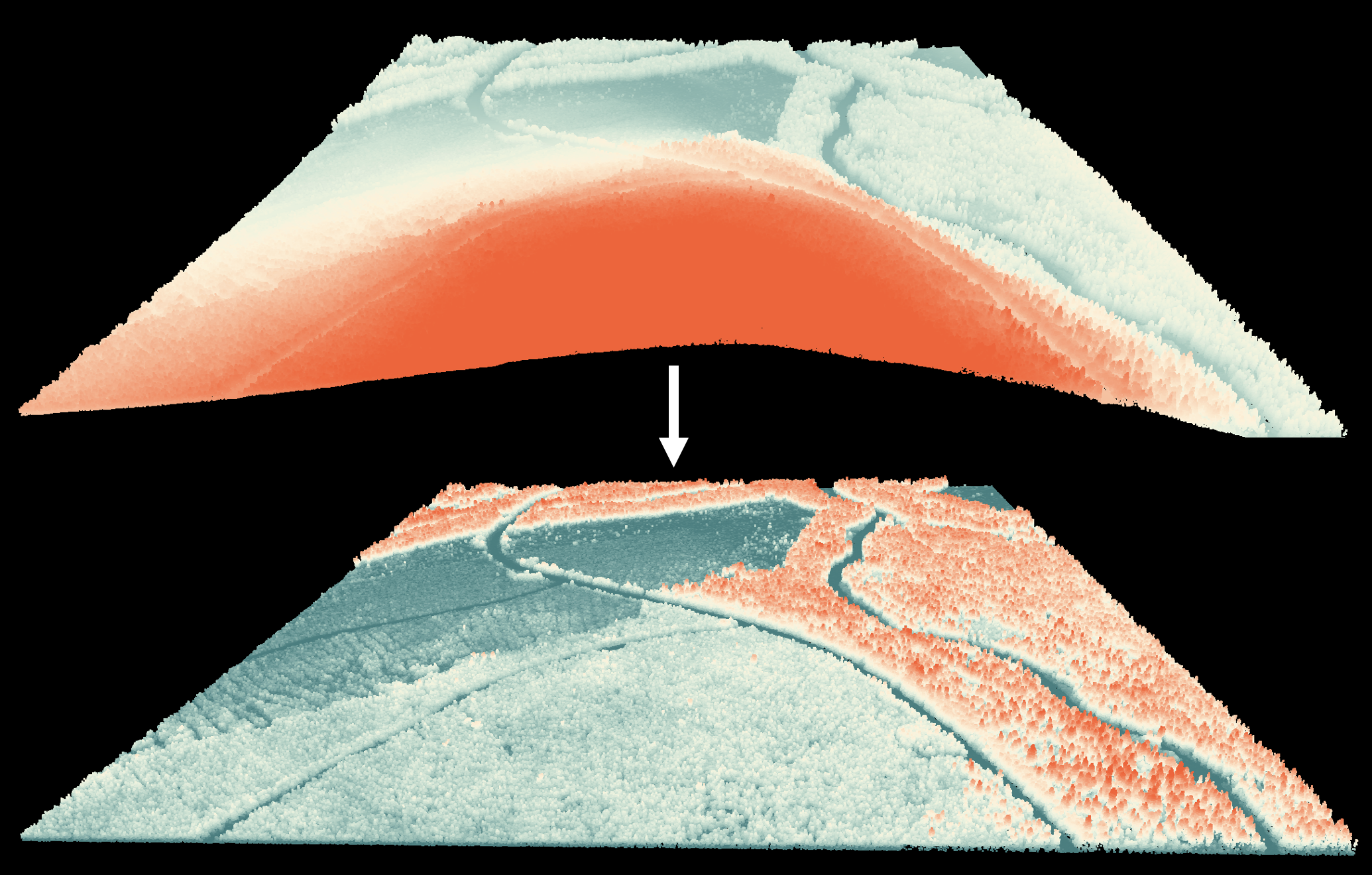
See Also: LidarTophatTransform, IndividualTreeDetection, LidarGroundPointFilter, ClassifyLidar
Parameters:
| Flag | Description |
|---|---|
| -i, --input | Name of the input LiDAR file |
| -o, --output | Name of the output LiDAR file |
| --dtm | Name of the input digital terrain model (DTM) raster file |
Python function:
wbt.normalize_lidar(
    i,
    output,
    dtm,
    callback=default_callback
)
Command-line Interface:
>> ./whitebox_tools -r=NormalizeLidar -i=points.laz ^
-o=normalized.laz --dtm=dtm.tif
Source code is unavailable due to proprietary license.
Author: Dr. John Lindsay
Created: 05/03/2023
Last Modified: 05/03/2023
RecoverFlightlineInfo
Note this tool is part of a WhiteboxTools extension product. Please contact Whitebox Geospatial Inc. for information about purchasing a license activation key (https://www.whiteboxgeo.com/extension-pricing/).
Raw airborne LiDAR data are collected along flightlines and multiple flightlines are typically merged into
square tiles to simplify data handling and processing. Commonly the Point Source ID attribute is used to
store information about the origin flightline of each point. However, sometimes this information is lost
(e.g. during data format conversion) or is omitted from some data sets. This tool can be used to identify
groups of points within a LiDAR file (--input) that belong to the same flightline.
The tool works by sorting points based on their timestamp and then identifying points for which the time
difference from the previous point is greater than a user-specified maximum time difference (--max_time_diff),
which are deemed to be the start of a different flightline. The operational assumption is that the time
between consecutive points within a flightline is usually quite small (usually a fraction of a second), while
the time between points in different flightlines is often relatively large (consider the aircraft turning time
needed to take multiple passes of the study area). By default the maximum time difference is set to 5.0
seconds, although it may be necessary to increase this value depending on the characteristics of a particular
data set.
The tool works on individual LiDAR tiles and the flightline identifiers will range from 0 to the number of
flightlines detected within the tile, minus one. Therefore, the flightline identifier created by this tool
will not extend beyond the boundaries of the tile and into adjacent tiles. That is, a flightline that extends
across multiple adjacent LiDAR tiles may have different flightline identifiers used in each tile. The identifiers
are intended to discriminate between flighlines within a single file. The flightline identifier value can
be optionally assigned to the Point Source ID point attribute (--pt_src_id), the User Data point attribute
(--user_data), and the red-green-blue point colour data (--rgb) within the output file (--output). At
least one of these output options must be selected and it is possible to select multiple output options.
Notice that if the input file contains any information within the selected output fields, the original
information will be over-written, and therefore lost--of course, it will remain unaltered within the input
file, which this tool does not modify. If the input file does not contain RGB colour data and
the --rgb output option is selected, the output file point format will be altered from the input file to
accommodate the addition of RGB colour data. Flightlines are assigned random colours. The LAS User Data point
attribute is stored as a single byte and, therefore, if this output option is selected and the input file
contains more than 256 flightlines, the tool will assign the same flightline identifier to more than one
flightline. It is very rare for this condition to be the case in a typical 1 km-square tiles. The Point Source ID
attribute is stored as a 16-bit integer and can therefore store 65,536 unique flightline identifiers.
Outputting flightline information within the colour data point attribute can be useful for visualizing areas of flightline overlap within a file. This can be an important quality assurance/quality control (QA/QC) step after acquiring a new LiDAR data set.
Please note that because this tool sorts points by their timestamps, the order of points in the output file may not match that of the input file.
See Also:
FlightlineOverlap, FindFlightlineEdgePoints, LidarSortByTime
Parameters:
| Flag | Description |
|---|---|
| -i, --input | Name of the input LiDAR points |
| -o, --output | Name of the output LiDAR points |
| --max_time_diff | Maximum in-flightline time difference (seconds) |
| --pt_src_id | Add flightline information to the point source ID |
| --user_data | Add flightline information to the user data |
| --rgb | Add flightline information to the RGB colour data |
Python function:
wbt.recover_flightline_info(
    i,
    output,
    max_time_diff=5.0,
    pt_src_id=False,
    user_data=False,
    rgb=False,
    callback=default_callback
)
Command-line Interface:
>> ./whitebox_tools -r=RecoverFlightlineInfo -i=input.las ^
-o=output.las --pt_src_id --rgb
Source code is unavailable due to proprietary license.
Author: Whitebox Geospatial Inc. (c)
Created: 12/02/2022
Last Modified: 13/02/2022
SelectTilesByPolygon
This tool copies LiDAR tiles overlapping with a polygon into an output directory. In actuality, the tool performs point-in-polygon operations, using the four corner points, the center point, and the four mid-edge points of each LiDAR tile bounding box and the polygons. This representation of overlapping geometry aids with performance. This approach generally works well when the polygon size is large relative to the LiDAR tiles. If, however, the input polygon is small relative to the tile size, this approach may miss some copying some tiles. It is advisable to buffer the polygon if this occurs.
See Also: LidarTileFootprint
Parameters:
| Flag | Description |
|---|---|
| --indir | Input LAS file source directory |
| --outdir | Output directory into which LAS files within the polygon are copied |
| --polygons | Input vector polygons file |
Python function:
wbt.select_tiles_by_polygon(
    indir,
    outdir,
    polygons,
    callback=default_callback
)
Command-line Interface:
>>./whitebox_tools -r=SelectTilesByPolygon -v ^
--indir='/path/to/lidar/' --outdir='/output/path/' ^
--polygons='watershed.shp'
Author: Dr. John Lindsay
Created: 01/08/2018
Last Modified: 19/05/2020
SortLidar
Note this tool is part of a WhiteboxTools extension product. Please contact Whitebox Geospatial Inc. for information about purchasing a license activation key (https://www.whiteboxgeo.com/extension-pricing/).
This tool can be used to sort the points in an input LiDAR file (--input) based on their properties
with respect to one or more sorting criteria (--criteria). The sorting criteria may include: the x, y or z
coordinates (x, y, z), the intensity data (intensity), the point class value (class), the point
user data field (user_data), the return number (ret_num), the point source ID (point_source_id), the
point scan angle data (scan_angle), the scanner channel (scanner_channel; LAS 1.4 datasets only), and
the acquisition time (time). The following is an example of a complex sorting criteria statement that
includes multiple criteria:
x 100.0, y 100.0, z 10.0, scan_angle
Criteria should be separated by a comma, semicolon, or pipe (|). Each criteria may have an associated bin value.
In the example above, point x values are sorted into bins of 100 m, which are then sorted by y values into bins
of 100 m, and sorted by point z values into bins of 10 m, and finally sorted by their scan_angle.
Sorting point values can have a significant impact on the compression rate when using certain compressed LiDAR data formats (e.g. LAZ, zLidar). Sorting values can also improve the visualization speed in some rendering software.
Note that if the user does not specify the optional input LiDAR file, the tool will search for all valid LiDAR (*.las, *.laz, *.zlidar) files contained within the current working directory. This feature can be useful for processing a large number of LiDAR files in batch mode. When this batch mode is applied, the output file names will be the same as the input file names but with a '_sorted' suffix added to the end.
See Also: LasToLaz, SplitLidar, FilterLidar, ModifyLidar
Parameters:
| Flag | Description |
|---|---|
| -i, --input | Name of the input LiDAR points |
| -o, --output | Name of the output LiDAR points |
| -c, --criteria | Sort criteria e.g. 'x 50.0, y 50.0, z'; criteria may include x, y, z, intensity, class, user_data, point_source_id, and scan_angle |
Python function:
wbt.sort_lidar(
    i=None,
    output=None,
    criteria="",
    callback=default_callback
)
Command-line Interface:
>> ./whitebox_tools -r=SortLidar -i=input.las ^
--criteria='x 100, y 100, z 10, time'
Source code is unavailable due to proprietary license.
Author: Whitebox Geospatial Inc. (c)
Created: 18/02/2022
Last Modified: 27/02/2022
SplitLidar
Note this tool is part of a WhiteboxTools extension product. Please contact Whitebox Geospatial Inc. for information about purchasing a license activation key (https://www.whiteboxgeo.com/extension-pricing/).
This tool can be used to split an input LiDAR file (--input) into a series of output files, placing
points into each output based on their properties with respect to a grouping criterion (--criterion).
Points can be grouped based on a specified the number of points in the output file (num_pts; note
the last file may contain fewer points), the x, y or z coordinates (x, y, z), the intensity data
(intensity), the point class value (class), the point user data field (user_data), the
point source ID (point_source_id), the point scan angle data (scan_angle), and the acquisition time
(time). Points are binned into groupings based on a user-specified interval value (--interval). For
example, if an interval of 50.0 is used with the z criterion, a series of files will be output that
are elevation bands of 50 m. The user may also optionally specify the minimum number of points needed before
a particular grouping file is saved (--min_pts). The interval value is not used for the class and
point_source_id criteria.
With this tool, a single input file can generate many output files. The names of the output files will be
reflective of the point attribute used for the grouping and the bin. For example, running the tool with the
on an input file named my_file.las using intensity criterion and with an interval of 1000 may produce the
following files:
- my_file_intensity0.las
- my_file_intensity1000.las
- my_file_intensity2000.las
- my_file_intensity3000.las
- my_file_intensity4000.las
Where the number after the attribute (intensity, in this case) reflects the lower boundary of the bin. Thus, the first file contains all of the input points with intensity values from 0 to just less than 1000.
Note that if the user does not specify the optional input LiDAR file, the tool will search for all valid LiDAR (*.las, *.laz, *.zlidar) files contained within the current working directory. This feature can be useful for processing a large number of LiDAR files in batch mode. When this batch mode is applied, the output file names will be the same as the input file names but with a suffix added to the end reflective of the split criterion and value (see above).
See Also: SortLidar, FilterLidar, ModifyLidar, LidarElevationSlice
Parameters:
| Flag | Description |
|---|---|
| -i, --input | Name of the input LiDAR points |
| --criterion | Criterion on which to base the split of the input file. Options include 'num_pts, 'x', 'y', 'z', intensity, 'class', 'user_data', 'point_source_id', 'scan_angle', 'time' |
| --interval | Interval |
| --min_pts | Minimum number of points in an output file |
Python function:
wbt.split_lidar(
    i=None,
    criterion="num_pts",
    interval="",
    min_pts=5,
    callback=default_callback
)
Command-line Interface:
>> ./whitebox_tools -r=SplitLidar -i=input.las --criterion=z ^
--interval=10.0 --min_pts=10
Source code is unavailable due to proprietary license.
Author: Whitebox Geospatial Inc. (c)
Created: 12/02/2022
Last Modified: 14/02/2022
ZlidarToLas
This tool can be used to convert one or more zLidar files ('*.zlidar') files into the LAS
LiDAR data format. zLidar files are a compressed
form of the LAS data format. The tool takes a list of input LAS files (--inputs). If --inputs
is unspecified, the tool will use all ZLidar files contained within the working directory
as the tool inputs. The user may also specify an optional output directory --outdir.
If this parameter is unspecified, each output LAS file will be written to the same
directory as the input files.
See Also: LasToZlidar, AsciiToLas
Parameters:
| Flag | Description |
|---|---|
| -i, --inputs | Input ZLidar files |
| --outdir | Output directory into which zlidar files are created. If unspecified, it is assumed to be the same as the inputs |
Python function:
wbt.zlidar_to_las(
    inputs=None,
    outdir=None,
    callback=default_callback
)
Command-line Interface:
>>./whitebox_tools -r=ZlidarToLas -v --wd="/path/to/data/" ^
-i="file1.zlidar, file2.zlidar, file3.zlidar"
Author: Dr. John Lindsay
Created: 13/05/2020
Last Modified: 13/05/2020